Assignment 7: R Plots, Regressions, and Functions
1 Accept Assignment on GitHub Classroom
Clone this assignment to your computer.
Restore the
renvpackage environment.
2 Regressions and Plots
2.1 Data
We will use the data from the package usdata.
The specific dataset will be usdata::county_complete which has a couple hundred different variables for U.S. states and counties.
Your goal is to write a regression model to predict “median_household_income_2019” using 5 other variables in the dataset.
2.2 Making Some Plots
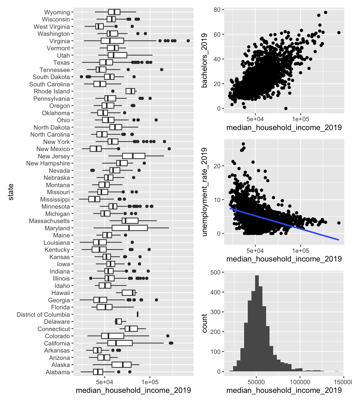
First make the following set of four plots using ggplot2
A histogram of “median_household_income_2019”
A scatter plot of “median_household_income_2019” and one of your 5 independent variables
A scatter plot of “median_household_income_2019” and another of your 5 independent variables
- Add a
geom_smooth()layer to this plot
- Add a
A boxplot with a box for each of the 50 U.S. states
Combining the plots
Now that you have made the plots,
- combine the plots together using
patchworkinto a single plot.
You should get something that looks like this (you can pick your own layout):
2.3 Fit Regressions
You will fit the following model, \[ Y = \beta_1 X_1 + \beta_2 X_2 + \beta_3 X_3 + \beta_4 X_4 + \beta_5 X_5 + \epsilon \]
where \(Y\) is median_houshold_income_2019 and each \(X_i\) are the other 5 variables you have chosen.
Use each of these three functions to fit the model:
lm()estimatr::lm_robust()fixest::feols()- one more model using
fixestwith a fixed effect for each state
2.4 Summarizing Regressions
Now,
- Combine the models using the
modelsummarypackage into a single table - Rename the models into something descriptive.
| lm | lm_robust | feols | feols_states | |
|---|---|---|---|---|
| (Intercept) | -3675.059 | -3675.059 | -3675.059 | |
| (2791.836) | (3116.996) | (2791.836) | ||
| unemployment_rate_2019 | -817.614 | -817.614 | -817.614 | -921.292 |
| (63.834) | (79.386) | (63.834) | (63.816) | |
| bachelors_2019 | 551.621 | 551.621 | 551.621 | 502.583 |
| (23.192) | (39.526) | (23.192) | (23.231) | |
| household_has_broadband_2019 | 699.844 | 699.844 | 699.844 | 641.646 |
| (24.749) | (27.116) | (24.749) | (24.202) | |
| hs_grad_2019 | -44.356 | -44.356 | -44.356 | -12.442 |
| (33.605) | (38.141) | (33.605) | (36.213) | |
| pop_2019 | 0.002 | 0.002 | 0.002 | 0.001 |
| (0.000) | (0.001) | (0.000) | (0.000) | |
| Num.Obs. | 3142 | 3142 | 3142 | 3141 |
| R2 | 0.648 | 0.648 | 0.648 | 0.718 |
| R2 Adj. | 0.647 | 0.647 | 0.647 | 0.713 |
| R2 Within | 0.603 | |||
| R2 Within Adj. | 0.602 | |||
| AIC | 65726.5 | 65726.5 | 65724.5 | 65097.9 |
| BIC | 65768.9 | 65768.9 | 65760.8 | 65430.8 |
| Log.Lik. | -32856.249 | |||
| RMSE | 8418.40 | 8418.40 | 8418.40 | 7526.29 |
| Std.Errors | IID | IID | ||
| FE: state | X |
2.5 Saving Output
Save 3 files to the “output” folder:
- A PDF of your combined plots (set the dimensions to be a full US letter page)
- A “.tex” file of the modelsummary table
- A “.md” file of the modelsummary table
3 Creating an R Package
This part of the assignment asks you to create a new R package with some basic functions and to then use that package in your assignment repository.
I recommend R Packagers (2e) as an invaluable resource and reference for learning how to make R packages.
3.1 Start a New GitHub Repository
You are going to make an R package that you are going to save and store on GitHub.
- Make a new GitHub repository, with the name you want for your package
- Make sure it’s public
- You could name it “testPackage” if you would like1
- Clone this new repository to your computer.
1 For R package names, avoid using special characters like “-” and “_” and spaces.
I am going to assume in these instructions that you named the package “testPackage”, but obviously if you named it something else, just replace the name.
3.2 Setup Your Package
Open up your local “testPackage” folder
Install “devtools”
In the terminal, run
usethis::create_package(".")
This will create the package files in the current folder.
Add a new R script called “myfunc.r” to the “R/” folder
Add the following code to that script:
testPackage/R/myfunc.r
#' My first function
#'
#' @param a A numerical vector.
#' @param b Also a numerical vector.
#'
#' @return A numerical vector of a + b * a.
#' @export
#'
#' @examples
#' myfunc(3, 5)
myfunc <- function(a, b) {
  result <- a * b + a
  return(result)
}
In the terminal, run
devtools::document()In the terminal, run
devtools::check()- Read the warning about the missing license
Add a license by running
usethis::use_mit_license()in the terminalRun
devtools::check()againCommit all the files, and push to GitHub
3.3 Install and Load Your Package
Now, we are going to see how we can use this package in other projetcs.
Switch back to your repository for this assignment (the one with the regression code and plots).
Since you made your package public on your GitHub account, you can install it using renv.
Install your package,
renv::install("yourGitHubUsername/testPackage")Check to see if the following code works:
library(testPackage)
myfunc(3, 5)
Can you access the help file for your function?2
Check to see if you can see “testPackage” in the “renv/” folder.
2 If you are having trouble, go to the “R” pane in VSCode and click on “Clear Cache and Restart Helper Server”.
3.4 Add to R Package: estimate_beta()
The task here is to write a new function to estimate \(\beta\) for a linear regression:
\[ y = \beta X + \epsilon \] \[ \Rightarrow \hspace{1cm} \widehat{\beta} = [X^\prime X]^{-1} X^\prime Y \]
Where \(y\) is a vector of \(n\) observations, \(X\) is a \(n\times k\) matrix of \(k\) variables, and \(\beta\) is a vector of \(k\) variables.
- Write a function
estimate_beta()- takes as inputs “y” and “X”
- returns “beta_hat”
3.5 Add to R Package: my_theme()
Write a function that retuns your favorite ggplot2 theme.
You’ll need to use usethis::use_package("ggplot2") to add ggplot2 as a dependency. You may possibly need to add other packages if you want to use one of their themes as a starting point.
You should make at least 3 adjustments to a default theme.
- Write a function
my_theme()- returns your
ggplot2theme
- returns your
3.6 Use estimate_beta() and my_theme()
Switching back to your assignment repository:
Use the
estimate_beta()function to estimate the \(\beta\) coefficients for one of your regression models.Use the
my_theme()function to change the theme of one of your plots.
4 Submit Your Assignment
Please add a link to your “testPackage” GitHub repository to the assignment’s README.md file.
Don’t forget to
renv::snapshot()the packages you are using!Commit all your changes to the assignment repository and push it
Navigate to the repository on GitHub and take a look at the “.md” output file of the regression table. It should render as a table on GitHub.