Optimization

Using programming languages to solve optimization problems

Matthew DeHaven

April 9, 2025

Course Home Page

Lecture Summary

Optimization
- Analytic
- Programmatic
  - Symbolic
  - Numeric
    - Grid Search
    - Gradient-free
    - Gradient-based
  - Automatic Differentiation

Quantecon

https://quantecon.org/lectures/

A super useful resource for learning about quantitative methods for solving economic models.

most lectures using Python, some using Julia
macro / finance focus
also a package of useful functions for Python and Julia

Optimization

Common Classes of Optimization Problems

Linear Programming (LP)
Quadratic Programing (QP)
Non-linear Programming (NLP)

There are efficient numerical methods for LP and some QP problems.

NLP problems are much harder.

R Packages for Each Class

LP: lpSolve
QP: quadprog
NLP: nloptr

We will be using nloptr today.

Numerical Optimization

Basic Macro Example

Let’s take a three equation macro model (with no stochastic shocks and no expectations). The Central Bank wants to minimize the loss function:

\[ i_t = \min_{i_t} \left( \pi_t - \pi^* \right)^2 \\ \pi_t = \kappa y_t \\ y_t = \chi i_t \]

Substituting in the Phillips curve and the IS curve, we have:

\[ i_t = \min_{i_t} \left( \kappa \chi i_t - \pi^* \right)^2 \]

Basic Macro Example

We know the FOC:

\[ \frac{\partial \mathbb{L}}{\partial i_t} = 0 = 2 \kappa \chi \left( \kappa \chi i_t - \pi^* \right) \\ i^* = \frac{1}{\kappa \chi} \pi^* \]

Which we can use to find the optimal interst rate for given values of \(\kappa\), \(\chi\), and \(\pi^*\).

If \(\kappa = 0.5\), \(\chi = 0.5\), and \(\pi^* = 2\), then: \[ i^* = \frac{1}{0.5 \cdot 0.5} \cdot 2 = 8 \]

Numerical Methods

This is a basic square-loss problem, but what if we could not use analytic methods?

Let’s look at some numerical methods that are available.

Grid Search
Gradient-free methods
Gradient-based methods

L = function(i) (0.5 * 0.5 * i - 2)^2

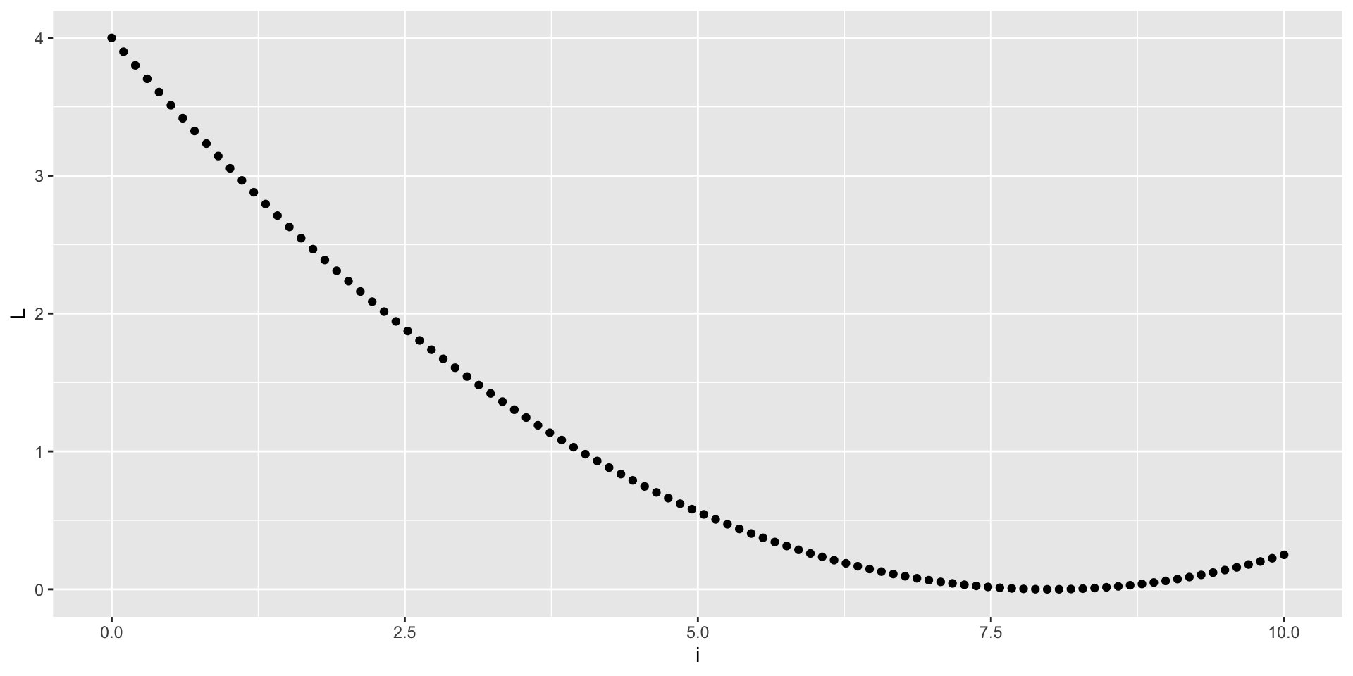
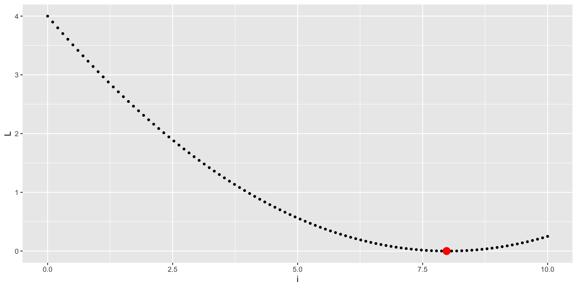
Grid Search

A grid search is a brute force method of searching for the optimal solution.

Define a grid of values for the variable of interest (in this case, \(i_t\))
Evaluate the loss function at each point in the grid
Find the point with the minimum value of the loss function
This is a very simple method, but it can be computationally expensive for large grids

Grid Search

library(ggplot2)


data.frame(
  i = seq(0, 10, length.out = 100),
  L = L(seq(0, 10, length.out = 100))
) |>
  ggplot(aes(x = i, y = L)) +
  geom_point()

Grid Search

library(ggplot2)
library(gghighlight)
data.frame(
  i = seq(0, 10, length.out = 100),
  L = L(seq(0, 10, length.out = 100))
) |>
  ggplot(aes(x = i, y = L)) +
  geom_point(color = "red", size = 4) +
  gghighlight(L == min(L), unhighlighted_params = list(color = "black", size = 1))

Gradient-free Methods

Gradient-free methods are useful when the loss function is not differentiable or when the gradient is difficult to compute.

One possible method is the Nelder-Mead method, which is a simplex-based optimization algorithm.

In general, gradient-free methods are less efficient than gradient-based methods.

Nonlinear Optimization in R: `nloptr`

nloptr is a package for nonlinear optimization and implements multiple methods.

library(nloptr)

opts <- list(
  "algorithm" = "NLOPT_LN_NELDERMEAD",
  "xtol_rel" = 0.0001,
  "maxeval" = 100
)

o <- nloptr(x0 = 0, eval_f = L, opts = opts)

Nelder-Mead Algorithm

The Nelder-Mead algorithm is a simplex-based optimization algorithm.

Construct a simplex of n+1 points in n-dimensional space
Evaluate the loss function at each point in the simplex
Reflect, expand, or contract the simplex based on the function values
Iterate until convergence

Nelder-Mead Method

opts <- list(
  "algorithm" = "NLOPT_LN_NELDERMEAD",
  "xtol_rel" = 0.0001,
  "maxeval" = 100
)

o <- nloptr(x0 = 0, eval_f = L, opts = opts)

o$iterations

[1] 32

o$solution

[1] 8

Gradient-based Methods

Gradient-based methods are more efficient than gradient-free methods, but they require the loss function to be differentiable.

One of the simplest gradient methods is Newton’s Method for optimization.

Requires us to know the gradient of the function.

dL = function(i) 2 * (0.5 * 0.5 * i - 2) * (0.5 * 0.5)

Newton’s Method for Optimization

Optimizes a function \(f(x)\) by finding roots for \(f^\prime(x)=0\).

Start with an initial guess \(x_0\)
Compute the gradient \(f^\prime(x_0)\)
Compute the Hessian \(f^{\prime\prime}(x_0)\)
Update the guess \(x_1 = x_0 - \frac{f\prime(x_0)}{f\prime\prime(x_0)}\)
Repeat until convergence

Some Restriction of Newton’s Method

Requires kndowledge of the gradient
Requires the Hessian to exist and be invertible

Quasi-Newton methods are a class of methods that approximate the Hessian.

BFGS is a popular quasi-Newton method that approximates the Hessian with changes in the gradient
Truncated Newton Method also approximates the Hessian

Truncated Newton’s Method

opts <- list(
  "algorithm" = "NLOPT_LD_TNEWTON",
  "xtol_rel" = 0.0001,
  "maxeval" = 100
)

o <- nloptr(x0 = 0, eval_f = L, eval_grad_f = dL, opts = opts)

o$iterations

[1] 3

o$solution

[1] 8

Numerical Gradient

Instead of computing the gradient analytically, we can use a numerical approximation.

dL_approx = function(i) nl.grad(i, fn = L)

This approximates the gradient using finite differences.

\[ f^\prime(x) \approx \frac{f(x + h) - f(x - h)}{2h} \]

where \(h\) is small.

Truncated Newton’s Method, numerical gradient

opts <- list(
  "algorithm" = "NLOPT_LD_TNEWTON",
  "xtol_rel" = 0.0001,
  "maxeval" = 100
)

o <- nloptr(x0 = 0, eval_f = L, eval_grad_f = dL_approx, opts = opts)

o$iterations

[1] 7

o$solution

[1] 8

Tracking the Iterations

It can be confusing to understand what is happening in the optimization process.

We can tell nloptr to save the intermediate values of the optimization process.

opts <- list(
  "algorithm" = "NLOPT_LN_NELDERMEAD",
  "xtol_rel" = 0.0001,
  "maxeval" = 100,
  "print_level" = 3
)
nloptr(x0 = 0, eval_f = L, opts = opts)

iteration: 1
    x = 0.000000
    f(x) = 4.000000
iteration: 2
    x = 1.000000
    f(x) = 3.062500
iteration: 3
    x = 2.000000
    f(x) = 2.250000
iteration: 4
    x = 3.000000
    f(x) = 1.562500
iteration: 5
    x = 5.000000
    f(x) = 0.562500
iteration: 6
    x = 7.000000
    f(x) = 0.062500
iteration: 7
    x = 11.000000
    f(x) = 0.562500
iteration: 8
    x = 9.000000
    f(x) = 0.062500
iteration: 9
    x = 11.000000
    f(x) = 0.562500
iteration: 10
    x = 8.000000
    f(x) = 0.000000
iteration: 11
    x = 7.000000
    f(x) = 0.062500
iteration: 12
    x = 8.500000
    f(x) = 0.015625
iteration: 13
    x = 7.500000
    f(x) = 0.015625
iteration: 14
    x = 8.250000
    f(x) = 0.003906
iteration: 15
    x = 7.750000
    f(x) = 0.003906
iteration: 16
    x = 8.125000
    f(x) = 0.000977
iteration: 17
    x = 7.875000
    f(x) = 0.000977
iteration: 18
    x = 8.062500
    f(x) = 0.000244
iteration: 19
    x = 7.937500
    f(x) = 0.000244
iteration: 20
    x = 8.031250
    f(x) = 0.000061
iteration: 21
    x = 7.968750
    f(x) = 0.000061
iteration: 22
    x = 8.015625
    f(x) = 0.000015
iteration: 23
    x = 7.984375
    f(x) = 0.000015
iteration: 24
    x = 8.007812
    f(x) = 0.000004
iteration: 25
    x = 7.992188
    f(x) = 0.000004
iteration: 26
    x = 8.003906
    f(x) = 0.000001
iteration: 27
    x = 7.996094
    f(x) = 0.000001
iteration: 28
    x = 8.001953
    f(x) = 0.000000
iteration: 29
    x = 7.998047
    f(x) = 0.000000
iteration: 30
    x = 8.000977
    f(x) = 0.000000
iteration: 31
    x = 7.999023
    f(x) = 0.000000
iteration: 32
    x = 8.000488
    f(x) = 0.000000


Call:
nloptr(x0 = 0, eval_f = L, opts = opts)


Minimization using NLopt version 2.10.0 

NLopt solver status: 4 ( NLOPT_XTOL_REACHED: Optimization stopped because 
xtol_rel or xtol_abs (above) was reached. )

Number of Iterations....: 32 
Termination conditions:  xtol_rel: 1e-04    maxeval: 100 
Number of inequality constraints:  0 
Number of equality constraints:    0 
Optimal value of objective function:  0 
Optimal value of controls: 8

Tracking the Iterations

nloptr does not return these intermediate values, but we can write some custom functions to capture them and clean them into a data.frame.

parse_optim_output <- function(text) {
  # Initialize vectors to store data
  iteration <- numeric()
  x <- numeric()
  fx <- numeric()
  
  # Process each group of 3 lines
  for(i in seq(1, length(text), 3)) {
    # Extract iteration number
    iter <- as.numeric(gsub("iteration: ", "", text[i]))
    
    # Extract x value using regex
    x_val <- as.numeric(gsub("\\s*\\tx = ", "", text[i+1]))
    
    # Extract function value
    f_val <- as.numeric(gsub("\\s*f\\(x\\) = ", "", text[i+2]))
    
    # Append values
    iteration <- c(iteration, iter)
    x <- c(x, x_val)
    fx <- c(fx, f_val)
  }
  
  # Create data.frame
  data.frame(
    iteration = iteration,
    x = x,
    fx = fx
  )
}

my_nloptr <- function(...){
  m <- capture.output({
    o <- nloptr(...)
  })

  df_m <- parse_optim_output(m)

  return(list(opt = o, iter = df_m))
}

Tracking the Iterations

opts <- list(
  "algorithm" = "NLOPT_LN_NELDERMEAD",
  "xtol_rel" = 0.0001,
  "maxeval" = 100,
  "print_level" = 3
)
o <- my_nloptr(x0 = 0, eval_f = L, eval_grad_f = dL, opts = opts)
o$iter

   iteration         x       fx
1          1  0.000000 4.000000
2          2  1.000000 3.062500
3          3  2.000000 2.250000
4          4  3.000000 1.562500
5          5  5.000000 0.562500
6          6  7.000000 0.062500
7          7 11.000000 0.562500
8          8  9.000000 0.062500
9          9 11.000000 0.562500
10        10  8.000000 0.000000
11        11  7.000000 0.062500
12        12  8.500000 0.015625
13        13  7.500000 0.015625
14        14  8.250000 0.003906
15        15  7.750000 0.003906
16        16  8.125000 0.000977
17        17  7.875000 0.000977
18        18  8.062500 0.000244
19        19  7.937500 0.000244
20        20  8.031250 0.000061
21        21  7.968750 0.000061
22        22  8.015625 0.000015
23        23  7.984375 0.000015
24        24  8.007812 0.000004
25        25  7.992188 0.000004
26        26  8.003906 0.000001
27        27  7.996094 0.000001
28        28  8.001953 0.000000
29        29  7.998047 0.000000
30        30  8.000977 0.000000
31        31  7.999023 0.000000
32        32  8.000488 0.000000

Visualizing the Iterations

library(gganimate)
ggplot(data = o$iter) +
  geom_function(fun = L) +
  geom_point(data = o$iter, aes(x = x, y = fx), color = "red", size = 4) +
  xlim(-2, 16) +
  transition_time(iteration) +
  shadow_mark(alpha = 0.2)

Comparing Methods

ggplot() +
  geom_function(fun = L) +
  geom_point(data = o_nm$iter, aes(x = x, y = fx, color = "NM"), size = 4, ) +
  geom_point(data = o_tn$iter, aes(x = x, y = fx, color = "TN"), size = 4) +
  xlim(-2, 16)

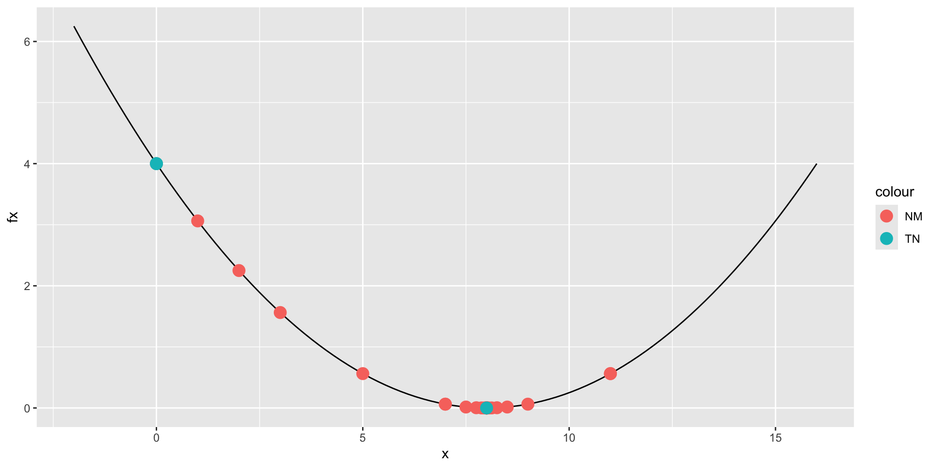
Local Minima

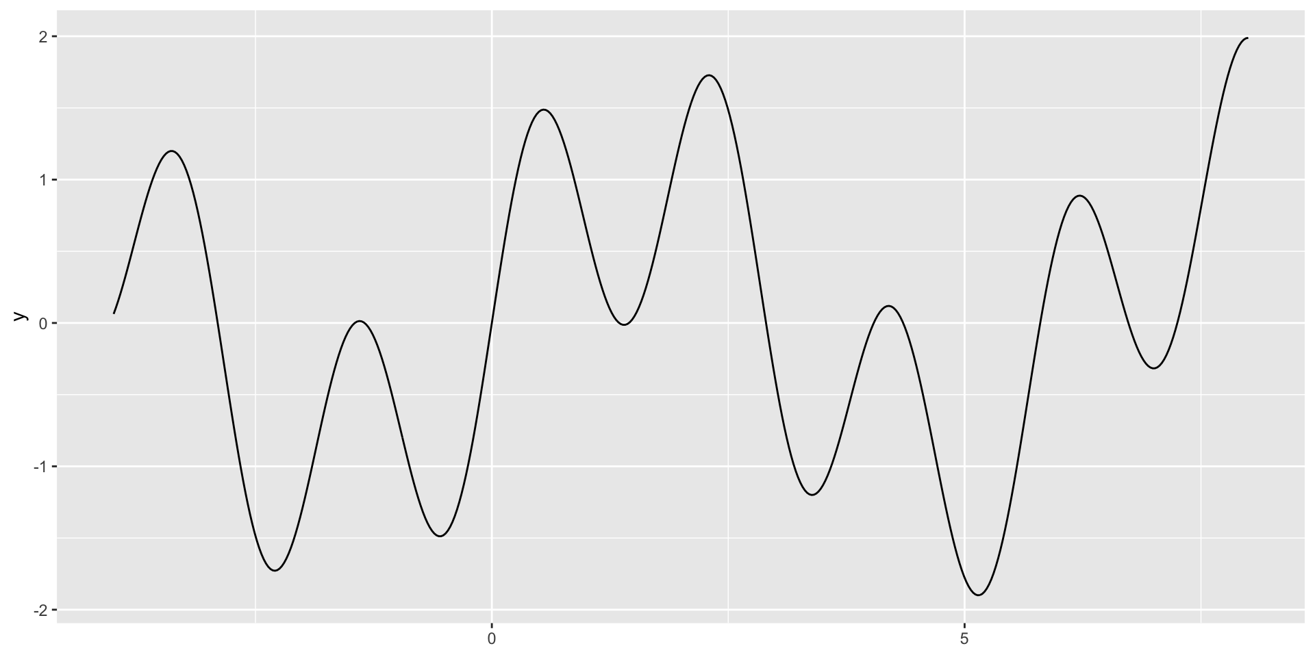
Let’s look at a more complicated example.

f <- function(x) sin(x) + sin((10.0 / 3.0) * x)
d <- function(x) cos(x) + (10.0 / 3.0) * cos((10.0 / 3.0) * x)

ggplot() +
  geom_function(fun = f, n = 500)  +
  xlim(-4, 8)

Numerical Approximation of Gradient

Again, we can use a numerical approximation of the gradient.

d_approx <- function(x) nl.grad(x, fn = f, heps = 0.5)

The argument heps is the step size for the numerical approximation.

setting heps to a large value to show the difference between using the numerical and analytical gradient

Calculating Minima

opts <- list(
  "algorithm" = "NLOPT_LN_NELDERMEAD",
  "xtol_rel" = 0.0001,
  "maxeval" = 100,
  "print_level" = 3
)
o_nm <- my_nloptr(x0 = 2, eval_f = f, opts = opts)

opts <- list(
  "algorithm" = "NLOPT_LD_TNEWTON",
  "xtol_rel" = 0.0001,
  "maxeval" = 100,
  "print_level" = 3
)
o_tn <- my_nloptr(x0 = 2, eval_f = f, eval_grad_f = d, opts = opts)

opts <- list(
  "algorithm" = "NLOPT_LD_TNEWTON",
  "xtol_rel" = 0.0001,
  "maxeval" = 100,
  "print_level" = 3
)
o_tn_approx <- my_nloptr(x0 = 2, eval_f = f, eval_grad_f = d_approx, opts = opts)

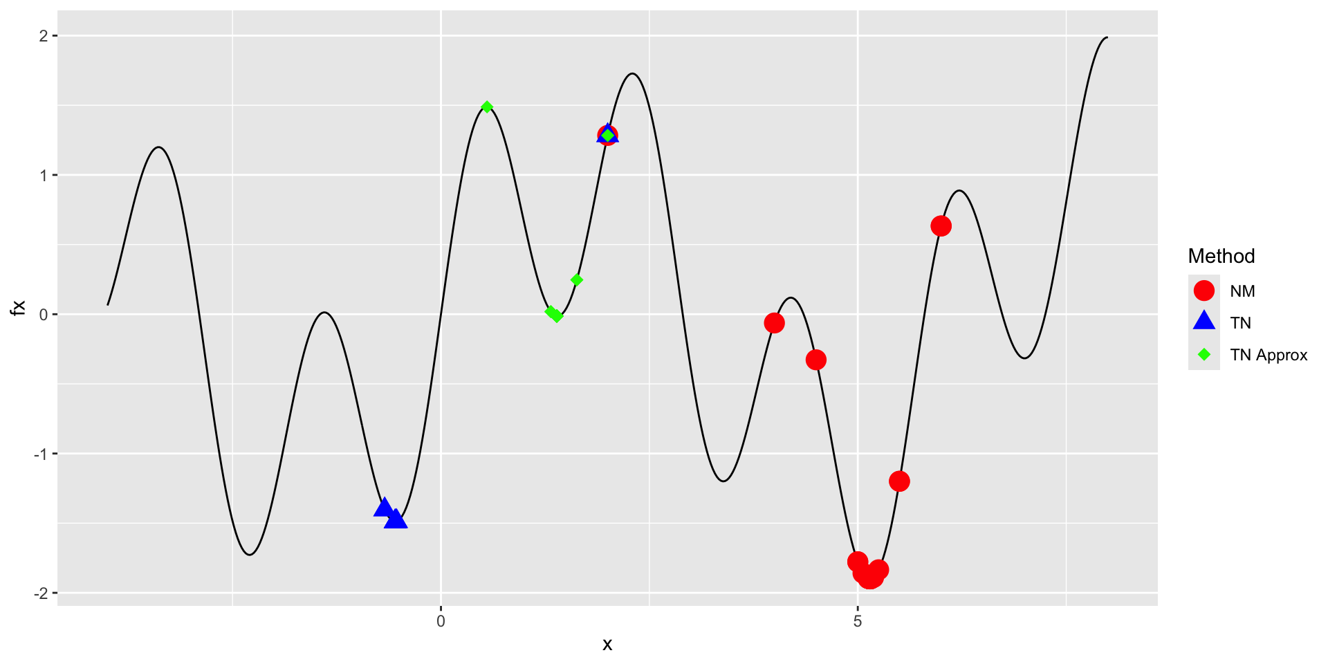
Comparing Methods

Solutions:

lapply(list(o_nm, o_tn, o_tn_approx), function(x) x$opt$solution)

[[1]]
[1] 5.145508

[[2]]
[1] -0.5488825

[[3]]
[1] 1.389585

Number of iterations:

lapply(list(o_nm, o_tn, o_tn_approx), function(x) max(x$iter$iteration))

[[1]]
[1] 26

[[2]]
[1] 11

[[3]]
[1] 28

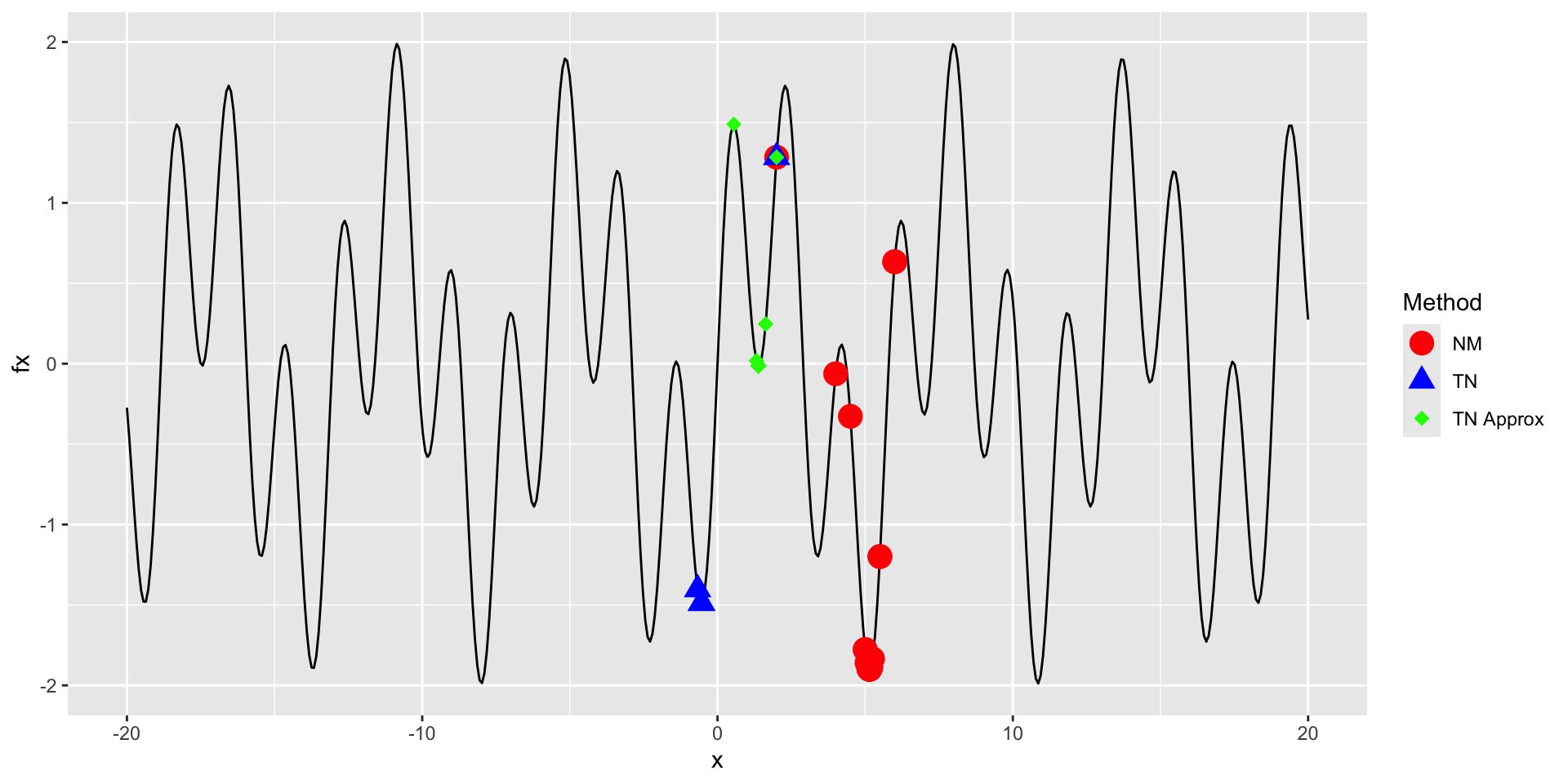
Zooming Out

All methods are finding local minima as this function is difficult to optimize.

Optimizing Over Multiple Arguments

So far we have been optimizing over a single variable.

But we can optimize over as many variables as we want.

f <- function(x) 2 * (x[1] - 1) ^ 2 + 5 * (x[2] - 3) ^ 2 + 10
d <- function(x) c(4 * (x[1] - 1), 10 * (x[2] - 3))

Graph the Function

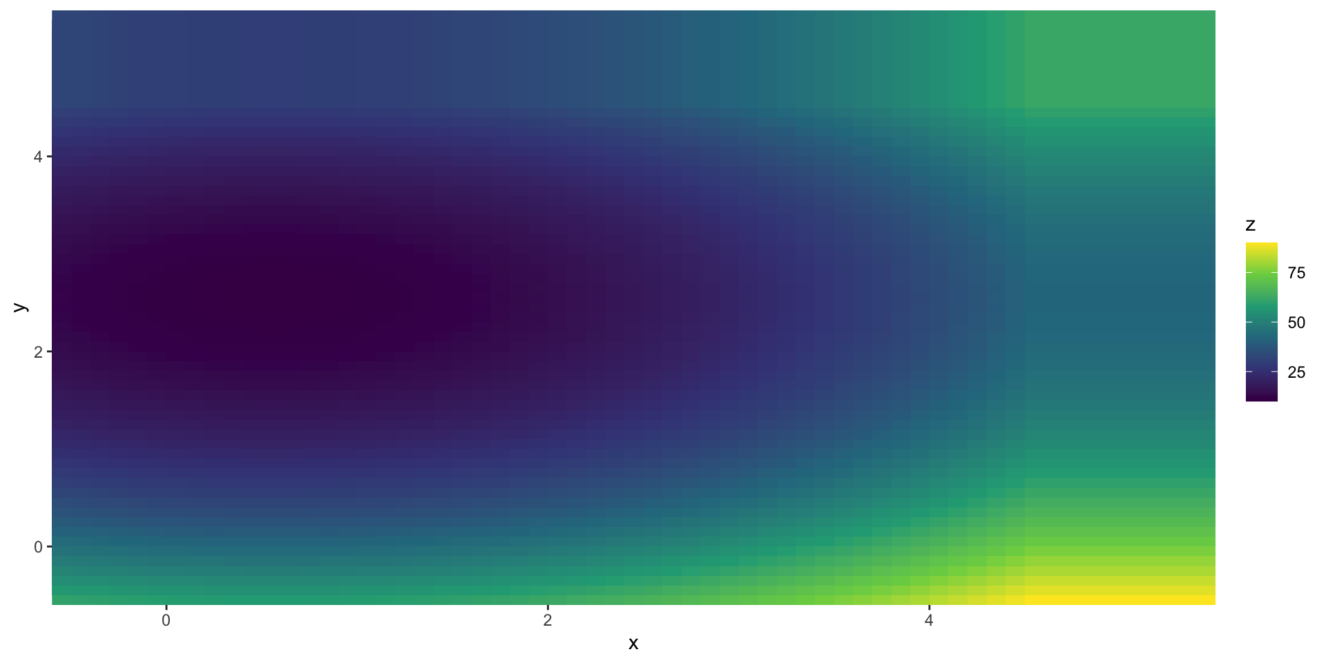
Optimizing Over Multiple Arguments

opts <- list(
  "algorithm" = "NLOPT_LD_TNEWTON",
  "xtol_rel" = 0.0001,
  "maxeval" = 100
)

nloptr(x0 = c(2, 2), eval_f = f, eval_grad_f = d, opts = opts)


Call:
nloptr(x0 = c(2, 2), eval_f = f, eval_grad_f = d, opts = opts)


Minimization using NLopt version 2.10.0 

NLopt solver status: 1 ( NLOPT_SUCCESS: Generic success return value. )

Number of Iterations....: 10 
Termination conditions:  xtol_rel: 1e-04    maxeval: 100 
Number of inequality constraints:  0 
Number of equality constraints:    0 
Optimal value of objective function:  10 
Optimal value of controls: 1 3

Visualizing the Iterations

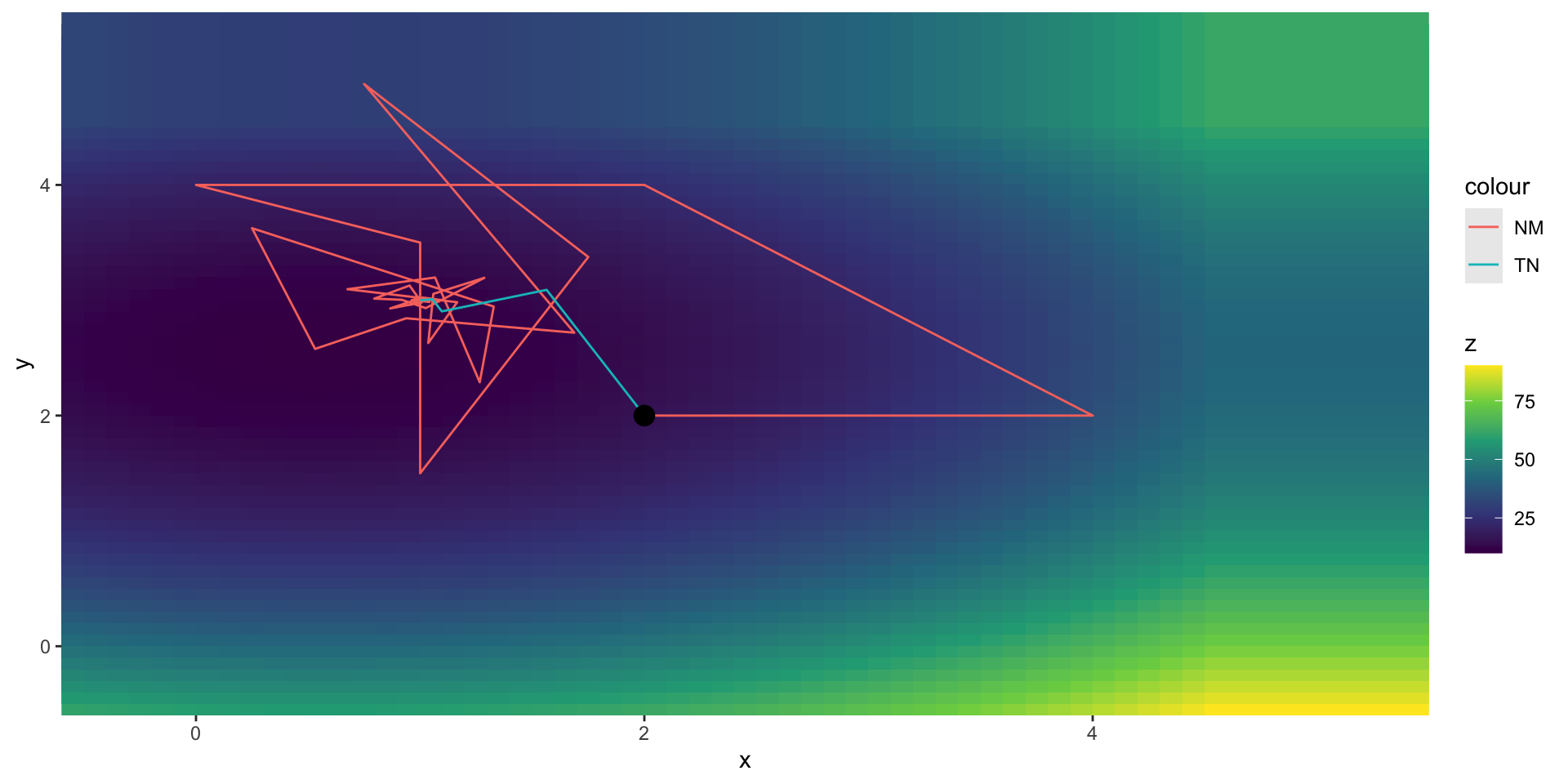
Comparing the Methods

lapply(list(o_nm, o_tn), function(x) x$opt$solution)

[[1]]
[1] 1.000071 2.999923

[[2]]
[1] 1 3

lapply(list(o_nm, o_tn), function(x) max(x$iter$iteration))

[[1]]
[1] 62

[[2]]
[1] 10

Numerical Optimization Overview

Grid Search
- Brute force, inefficient, good at global optima
Gradient-free methods
- less efficient, good for non-differentiable functions
Gradient-based methods
- more efficient, requires an analytic or numeric gradient

Solving Optimization Problems

Generally, you try to solve an optimization problem by…

Finding an analytic solution by hand
Finding an analytic solution with a Symbolic engine
Numerical optimization
- gradient-based method
- grid search

When turning to numerical optimization, the key is finding or approximating the gradient.

automatic differentiation (AD) is another method for calculating the gradient of a function

Symbolic Optimization

What is Symbolic Optimization?

When you solve an optimization problem by hand, you apply a set of rules to find the gradient, then rearrange the FOC to find zero roots.

A symbolic engine emulates this same process.

Mathematica is an example of a common symbolic engine

Python has a great symbolic engine called SymPy which we will take a look at.

Automatic Differentiation

What is Automatic Differentiation?

We have so far seen two ways to calculate the gradient of a function:

Analytically (or symbollically)
Finite differences (approximation up to some order ‘n’)

Automatic differentiation (AD)
- a method for calculating the derivative of a function using the chain rule

AD Chain Rule

\[ \begin{align*} y &= f(g(h(x))) = f(g(h(w_0))) = f(g(w_1)) = f(w_2) \\ w_0 &= x \\ w_1 &= h(w_0) \\ w_2 &= g(w_1) \\ w_3 &= f(w_2) = y \\ \frac{dy}{dx} &= \frac{dy}{dw_2} \cdot \frac{dw_2}{dw_1} \cdot \frac{dw_1}{dx} \\ &= \frac{df(w_2)}{dw_2} \cdot \frac{dg(w_1)}{dw_1} \cdot \frac{dh(w_0)}{dw_0} \end{align*} \]

The “trick” of AD is that we can build up complicated composite functions as a series of partial derivatives of each step.

Forward vs. Reverse Mode AD

\[ \frac{dy}{dx} = \frac{dy}{dw_2} \cdot \frac{dw_2}{dw_1} \cdot \frac{dw_1}{dx} \]

Forward AD calculates:

\(\frac{dw_1}{dx}\) then \(\frac{dw_2}{dw_1}\) then \(\frac{dy}{dw_2}\)

Reverse AD calculates:

\(\frac{dy}{dw_2}\) then \(\frac{dw_2}{dw_1}\) then \(\frac{dw_1}{dx}\)

Forward vs. Reverse Mode AD

Given a function \(f: \mathbb{R}^n \to \mathbb{R}^m\)

if \(n << m\), then forward mode is more efficient
if \(n >> m\), then reverse mode is more efficient

For a loss function, \(f: \mathbb{R}^n \to \mathbb{R}\), so reverse mode is more efficient.

A Simple AD example

\[ \begin{align*} f(x_1, x_2) &= x_1 x_2 + sin(x_1) \\ &= w_1 + w_2 \\ &= w_3 \\ \frac{dy}{dx} &= \frac{dw_3}{dw_1} \cdot \frac{dw_1}{dx} + \frac{dw_3}{dw_2} \cdot \frac{dw_2}{dx} \end{align*} \]

In this example, each step is easy to calculate:

\[ \frac{dy}{dx} = \underbrace{\frac{dw_3}{dw_1}}_{1} \cdot \underbrace{\frac{dw_1}{dx}}_{x_1 + x_2} + \underbrace{\frac{dw_3}{dw_2}}_{1} \cdot \underbrace{\frac{dw_2}{dx}}_{cos(x_1)} \]

Because this problem was simple, when we follow the AD chain rule, we derive the symbolic solution.

AD vs. Symbolic Differentiation

AD, however, can be used in many cases where symbolic differentiation is not possible.

Automatic Differentiation is usually calculated only for a single point at a time, not for the entire function.

This means it can handle functions that

are not differentiable everywhere
cannot be “written down”
are not continuous

AD does require that a function can be written programmatically/algorithmically.

AD in Machine Learning

Automatic Differeneiation is the key step behind fitting large neural networks.

Neural networks have the following features/goals:

A loss function with many paramaeters: \(f: \mathbb{R}^n \to \mathbb{R}\)
Can be written programmatically, but not symbolically
Cares about precision and efficiency
But doesn’t care about a closed-form expression of the gradient

More AD Resources

What’s Automatic Differentiation? by Andrew Holmes
Automatic Differentation Wikipedia
Automatic Differentation JAX Python Documentation

Summary

Lecture Summary

Optimization
- Analytic
- Programmatic
  - Symbolic
  - Numeric
    - Grid Search
    - Gradient-free
    - Gradient-based
  - Automatic Differentiation

Live Coding Example

Python Sympy Coding Example (symoblic)
Python JAX Coding Example (automatic differentiation)

Optimization

Lecture Summary

Quantecon

Optimization

Common Classes of Optimization Problems

R Packages for Each Class

Numerical Optimization

Basic Macro Example

Basic Macro Example

Numerical Methods

Grid Search

Grid Search

Grid Search

Gradient-free Methods

Nonlinear Optimization in R: nloptr

Nelder-Mead Algorithm

Nelder-Mead Method

Gradient-based Methods

Newton’s Method for Optimization

Some Restriction of Newton’s Method

Truncated Newton’s Method

Numerical Gradient

Truncated Newton’s Method, numerical gradient

Tracking the Iterations

Tracking the Iterations

Tracking the Iterations

Visualizing the Iterations

Comparing Methods

Local Minima

Numerical Approximation of Gradient

Calculating Minima

Comparing Methods

Comparing Methods

Zooming Out

Optimizing Over Multiple Arguments

Graph the Function

Optimizing Over Multiple Arguments

Visualizing the Iterations

Comparing the Methods

Numerical Optimization Overview

Solving Optimization Problems

Symbolic Optimization

What is Symbolic Optimization?

Automatic Differentiation

What is Automatic Differentiation?

AD Chain Rule

Forward vs. Reverse Mode AD

Forward vs. Reverse Mode AD

A Simple AD example

AD vs. Symbolic Differentiation

AD in Machine Learning

More AD Resources

Summary

Lecture Summary

Live Coding Example

Nonlinear Optimization in R: `nloptr`