Symbolic Math with SymPy

Author

Matthew DeHaven

Install Sympy

terminal

pip install sympy

import sympy as sp
sp.init_printing() ## Makes output pretty

Take a simple Macro model where a central bank tries to minimize inflation \(\pi\) and the output gap \(y\).

\[ \begin{align*} i_t &= \min_{i_t} \left( \pi_t - \pi^* \right)^2 + \left( y_t \right)^2 \\ \pi_t &= \kappa y_t \\ y_t &= \chi i_t \end{align*} \]

We can write this in Python using SymPy:

y, π, i, π_star, κ, Χ = sp.symbols('y π i π^* κ Χ')

y = Χ * i
π = κ * y
loss = (π - π_star) ** 2 + y ** 2


loss

\(\displaystyle i^{2} Χ^{2} + \left(i Χ κ - π^{*}\right)^{2}\)

And now we can take an symbolic derivative…

d_loss = sp.diff(loss, i)
d_loss

\(\displaystyle 2 i Χ^{2} + 2 Χ κ \left(i Χ κ - π^{*}\right)\)

And then solve \(\frac{d L}{d i} = 0\) for \(i\):

i_opt = sp.solve(d_loss, i)
i_opt

\(\displaystyle \left[ \frac{κ π^{*}}{Χ \left(κ^{2} + 1\right)}\right]\)

Which is our optimal value for the interest rate!

We can substitute in values for the parameters to get a numeric result:

i_opt_numeric = i_opt[0].subs({κ: 0.5, Χ: 0.5, π_star: 0.02})
i_opt_numeric

\(\displaystyle 0.016\)

Another simple example, with the Solow Growth Model.

\[ k_{t+1} = s A k_t^\alpha + (1 - \delta) k_t \]

A, s, k, α, δ = sp.symbols('A s k^* α δ')
kp = s * A * k ** α + (1 - δ) * k - k
solow = sp.Eq(kp, 0)
solow

\(\displaystyle A \left(k^{*}\right)^{α} s + k^{*} \left(1 - δ\right) - k^{*} = 0\)

Let’s solve for \(k_{t+1} = k_t = k^*\):

k_star = sp.solve(solow, k)
k_star

\(\displaystyle \left[ \left(\frac{A s}{δ}\right)^{- \frac{1}{α - 1}}\right]\)

And if we have some parameters for our Solow model, we could substitute them in:

params = {A: 1, s: 0.2, α: 0.5, δ: 0.1}
k_star_numeric = k_star[0].subs(params)
k_star_numeric

\(\displaystyle 4.0\)

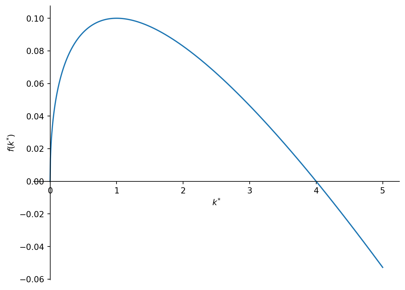
And we could graph the function for \(k_{t+1}\):

sp.plot(kp.subs(params), (k, 0, 5))