library(fredr)
fredr_set_key(fred_api_key)R Databases and APIs
Using Fred
The package I suggest using to download data from FRED:
You will need to get your own API key from FRED here.
Then add a line of code to your srcipt:
fred_api_key <- "YOUR KEY HERE"If you haven’t already, install the two packages in your terminal:
renv::install("fredr")
renv::install("alfred")
fredr
Load the package and then set the key for this session.
Download data
To download one series:
unemp <- fredr(series_id = "UNRATE")For multiple series, use the purrr::map_dfr() function:
data <- purrr::map_dfr(c("UNRATE", "FEDFUNDS"), fredr)And now we can make a quick chart of the data.
library(ggplot2)

data |>
  ggplot(aes(x = date, y = value, color = series_id)) + geom_line()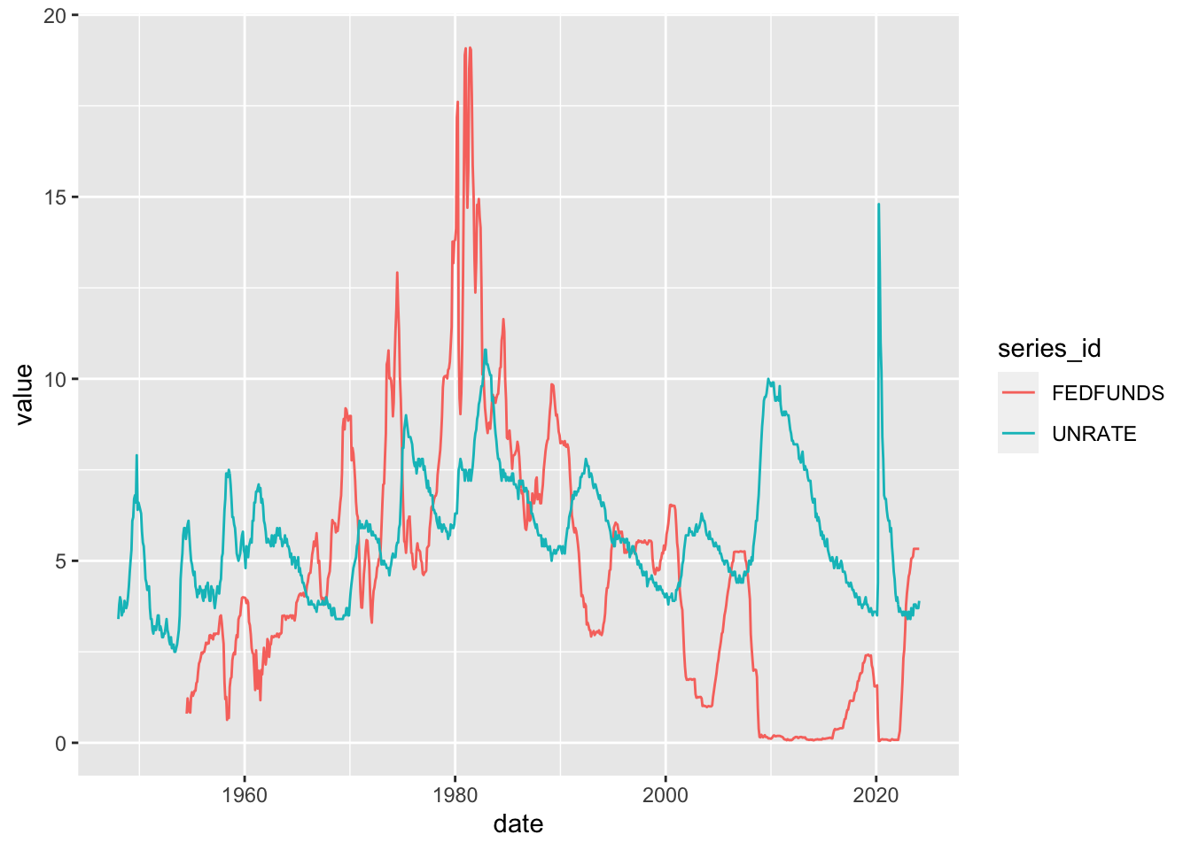
fredr options
You can set a lot of options for fredr:
library(dplyr)

rgdp <- fredr(
  "GDPC1",
  observation_start = as.Date("2000-01-01"),
  observation_end = as.Date("2024-01-01"),
  frequency = "q", # quarterly
  units = "pc1"    # percent change from 1 year ago
  )

rgdp |>
  ggplot(aes(x = date, y = value, fill = series_id)) + geom_col()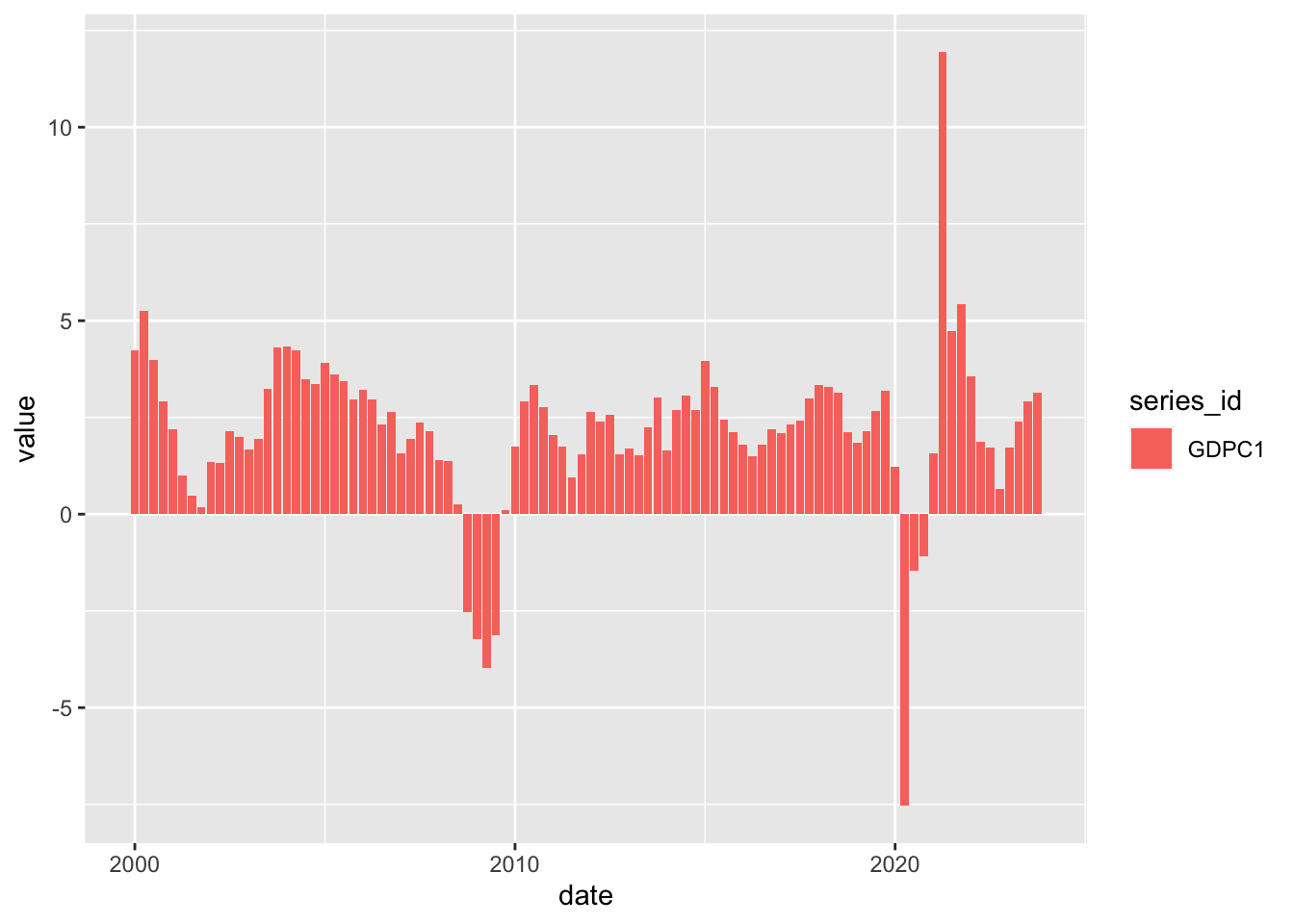
Vintage data
Data gets revised overtime, usually just by a small amount, but sometimes the changes can be quite large. The data series for GDP in particular gets lots of revisions.
You can access data from any point in time on FRED by setting the “vintage_dates=” argument in the function call.
For instance, here we pull data on GDP growth for the year 2022, once with values known on “2023-02-01” and then at “2023-06-01”.
rgdp_vintage1 <- fredr(
  "GDPC1",
  observation_start = as.Date("2022-01-01"),
  observation_end = as.Date("2022-12-31"),
  vintage_dates = as.Date("2023-02-01"),
  frequency = "q",
  units = "pc1"
  )

rgdp_vintage2 <- fredr(
  "GDPC1",
  observation_start = as.Date("2022-01-01"),
  observation_end = as.Date("2022-12-31"),
  vintage_dates = as.Date("2023-06-01"),
  frequency = "q",
  units = "pc1"
  )

rbind(rgdp_vintage1, rgdp_vintage2) |>
  ggplot(aes(x = date, y = value, fill = as.factor(realtime_start))) +
  geom_col(position = "dodge")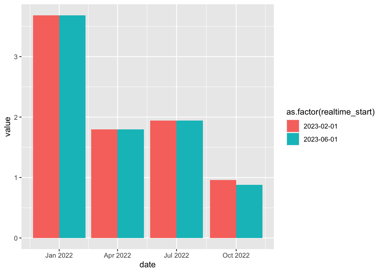
You can see the revision in the fourth quarter of the GDP growth data for 2022.
tidycensus
There are a few different R packages for talking accessing the U.S. census data.
Go ahead and install the tidycensus package.
renv::install("tidycensus")To get the install to work I had to install both gdal and udunits using homebrew.
library(tidycensus)
library(tidyverse)
You will need to have another API key for the census which you can get here: http://api.census.gov/data/key_signup.html.
Yes it does look like a fake website, but it’s actually the Census.
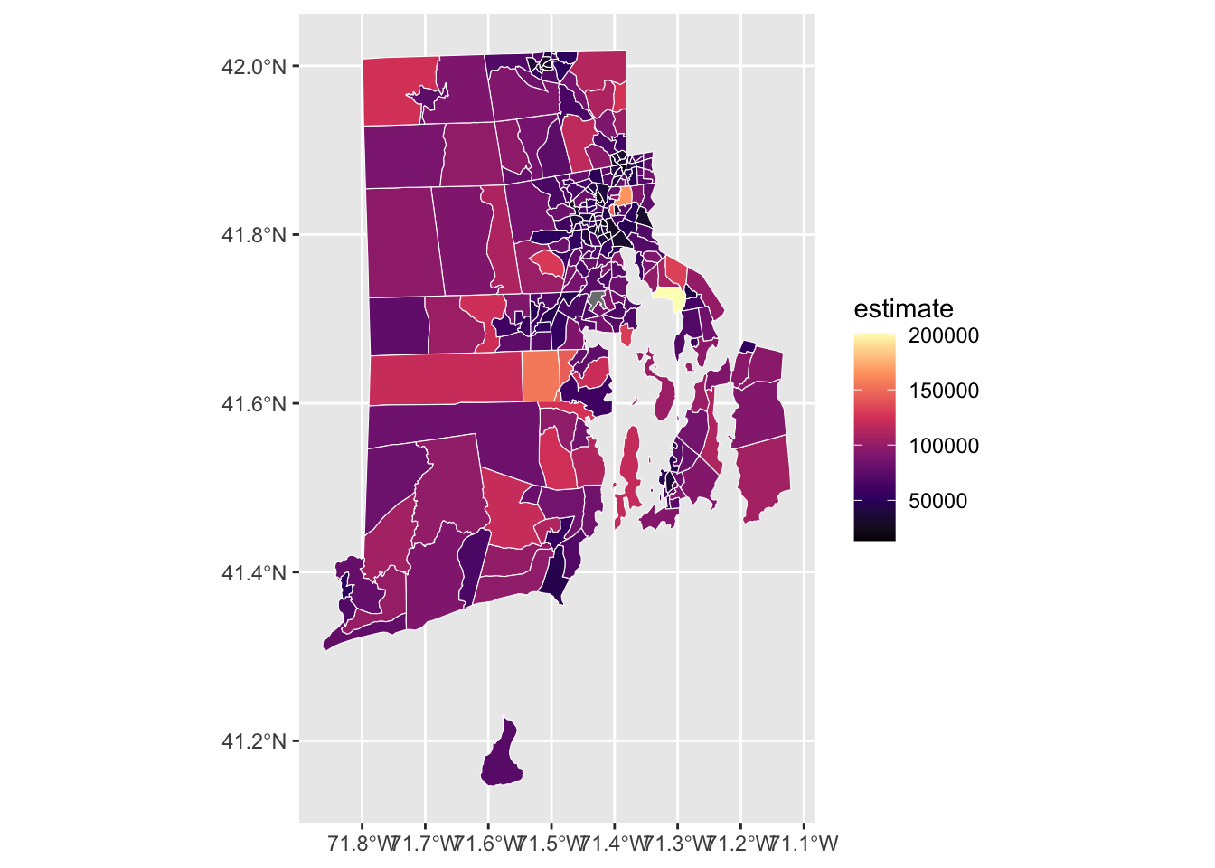
census_api_key("YOUR API KEY GOES HERE")We can pull data from the ACS on median household income by Census tract.
ri <- get_acs(
  state = "RI",
  geography = "tract",
  variables = "B19013_001",
  geometry = TRUE,
  year = 2020
)
Getting data from the 2016-2020 5-year ACSDownloading feature geometry from the Census website. To cache shapefiles for use in future sessions, set `options(tigris_use_cache = TRUE)`.
  |
  |                                                                      |   0%
  |
  |==========                                                            |  14%
  |
  |====================                                                  |  28%
  |
  |=============================                                         |  42%
  |
  |=======================================                               |  56%
  |
  |=================================================                     |  70%
  |
  |====================================================================  |  98%
  |
|======================================================================| 100%riSimple feature collection with 250 features and 5 fields (with 3 geometries empty)
Geometry type: MULTIPOLYGON
Dimension: XY
Bounding box: xmin: -71.86277 ymin: 41.14634 xmax: -71.12057 ymax: 42.0188
Geodetic CRS: NAD83
First 10 features:
GEOID NAME variable
1 44001030100 Census Tract 301, Bristol County, Rhode Island B19013_001
2 44003021600 Census Tract 216, Kent County, Rhode Island B19013_001
3 44003020101 Census Tract 201.01, Kent County, Rhode Island B19013_001
4 44005040800 Census Tract 408, Newport County, Rhode Island B19013_001
5 44007014100 Census Tract 141, Providence County, Rhode Island B19013_001
6 44007010200 Census Tract 102, Providence County, Rhode Island B19013_001
7 44007000400 Census Tract 4, Providence County, Rhode Island B19013_001
8 44007011800 Census Tract 118, Providence County, Rhode Island B19013_001
9 44007011100 Census Tract 111, Providence County, Rhode Island B19013_001
10 44007001200 Census Tract 12, Providence County, Rhode Island B19013_001
estimate moe geometry
1 99167 11319 MULTIPOLYGON (((-71.3539 41...
2 130104 25333 MULTIPOLYGON (((-71.39157 4...
3 71932 7447 MULTIPOLYGON (((-71.53322 4...
4 72209 10138 MULTIPOLYGON (((-71.31293 4...
5 39652 16124 MULTIPOLYGON (((-71.45225 4...
6 51349 9094 MULTIPOLYGON (((-71.38557 4...
7 43456 25844 MULTIPOLYGON (((-71.42086 4...
8 48259 17241 MULTIPOLYGON (((-71.44129 4...
9 31393 4611 MULTIPOLYGON (((-71.40705 4...
10 40380 6980 MULTIPOLYGON (((-71.43134 4...And with ggplot2, this is extremely easy to plot!
ri %>%
  ggplot(aes(fill = estimate)) +
  geom_sf(color = "white") +
  scale_fill_viridis_c(option = "magma")