Assignment 4: R Plots and Regressions

1 Accept Assignment on Github Classroom

1. Accept Assignment 4 on Github Classroom.

2. Clone this assignment to your computer.

3. Restore the renv package environment.

2 Data

We will use the data from the package usdata.

The specific dataset will be usdata::county_complet which has a couple hundred different variables for U.S. states and counties.

Your goal is to write a regression model to predict “median_household_income_2019” using 5 other variables in the dataset.

`modelsummary` 2.0.0 now uses `tinytable` as its default table-drawing
  backend. Learn more at: https://vincentarelbundock.github.io/tinytable/

Revert to `kableExtra` for one session:

  options(modelsummary_factory_default = 'kableExtra')

Change the default backend persistently:

  config_modelsummary(factory_default = 'gt')

Silence this message forever:

  config_modelsummary(startup_message = FALSE)

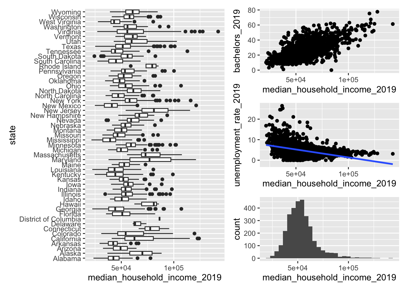
3 Making Some Plots

First make the following set of four plots using ggplot2

• A histogram of “median_household_income_2019”

• A scatter plot of “median_household_income_2019” and one of your 5 independent variables

• A scatter plot of “median_household_income_2019” and another of your 5 independent variables

  • Add a geom_smooth() layer to this plot

• A boxplot with a box for each of the 50 U.S. states

Combining the plots

Now that you have made the plots,

• combine the plots together using patchwork into a single plot.

You should get something that looks like this (you can pick your own layout):

4 Fit Regressions

You will fit the following model, \[ Y = \beta_1 X_1 + \beta_2 X_2 + \beta_3 X_3 + \beta_4 X_4 + \beta_5 X_5 + \epsilon \]

where \(Y\) is median_houshold_income_2019 and each X are the other 5 variables you have chosen.

Use each of these three functions to fit the model:

• lm()
• estimatr::lm_robust()
• fixest::feols()

And then,

• fit one more model using fixest where you add a fixed effect for each state.

Summarizing Regressions

Now,

• Combine the models using modelsummary into a single table.
  • Rename the models into something descriptive.

	lm	lm_robust	feols	feols_states
(Intercept)	-3675.059	-3675.059	-3675.059
	(2791.836)	(3116.996)	(2791.836)
unemployment_rate_2019	-817.614	-817.614	-817.614	-921.292
	(63.834)	(79.386)	(63.834)	(140.713)
bachelors_2019	551.621	551.621	551.621	502.583
	(23.192)	(39.526)	(23.192)	(53.375)
household_has_broadband_2019	699.844	699.844	699.844	641.646
	(24.749)	(27.116)	(24.749)	(41.326)
hs_grad_2019	-44.356	-44.356	-44.356	-12.442
	(33.605)	(38.141)	(33.605)	(63.125)
pop_2019	0.002	0.002	0.002	0.001
	(0.000)	(0.001)	(0.000)	(0.001)
Num.Obs.	3142	3142	3142	3142
R2	0.648	0.648	0.648	0.719
R2 Adj.	0.647	0.647	0.647	0.714
R2 Within				0.603
R2 Within Adj.				0.602
AIC	65726.5	65726.5	65724.5	65119.6
BIC	65768.9	65768.9	65760.8	65458.5
Log.Lik.	-32856.249
RMSE	8418.40	8418.40	8418.40	7525.09
Std.Errors			IID	by: state
FE: state				X

5 Saving Output

You need to save 3 files to the “output” folder.

• A PDF of your combined plots (set the dimensions to be a full US letter page)
• A “.tex” file of the modelsummary table
• A “.md” file of the modelsummary table

6 Push To Github

Don’t forget to renv::snapshot() the packages you are using!

If you haven’t already, commit everything and push to Github.

• Navigate to the repository on Github and take a look at the “.md” output file of the regression table. It should render as a table on Github.