Key: <state_code, state_text>
    state_code           state_text    HI    JO    LD    OS    QU    TS    UO
        <char>               <char> <num> <num> <num> <num> <num> <num> <num>
 1:         00             Total US  3.76  4.27  1.29  0.23  2.10  3.64  1.70
 2:         01              Alabama  3.96  4.21  1.22    NA  2.27  3.75  1.70
 3:         02               Alaska  5.66  5.75  2.10    NA  3.23  5.75  1.31
 4:         04              Arizona  4.24  4.62  1.29    NA  2.53  4.05  1.78
 5:         05             Arkansas  4.07  4.19  1.26    NA  2.39  3.91  1.56
 6:         06           California  3.38  3.99  1.24    NA  1.83  3.31  2.37
 7:         08             Colorado  4.27  4.54  1.44    NA  2.47  4.16  1.48
 8:         09          Connecticut  3.11  3.73  1.22    NA  1.53  2.98  2.10
 9:         10             Delaware  4.51  4.56  1.46    NA  2.55  4.29  1.35
10:         11 District of Columbia  2.72  3.61  0.92    NA  1.53  2.69  1.08
11:         12              Florida  3.86  4.27  1.28    NA  2.24  3.76  1.85
12:         13              Georgia  4.30  4.66  1.39    NA  2.51  4.18  1.84
13:         15               Hawaii  3.50  3.96  1.20    NA  1.97  3.39  1.39
14:         16                Idaho  4.61  4.68  1.48    NA  2.59  4.35  1.32
15:         17             Illinois  3.69  4.13  1.29    NA  1.96  3.47  2.05
16:         18              Indiana  4.08  4.13  1.43    NA  2.33  3.98  1.65
17:         19                 Iowa  3.51  4.14  1.19    NA  2.01  3.42  1.16
18:         20               Kansas  3.61  4.18  1.19    NA  2.11  3.55  1.29
19:         21             Kentucky  4.29  4.55  1.36    NA  2.49  4.11  1.59
20:         22            Louisiana  4.24  4.32  1.39    NA  2.53  4.20  1.64
21:         23                Maine  3.84  4.49  1.53    NA  1.94  3.76  1.34
22:         24             Maryland  3.47  4.56  1.23    NA  1.94  3.44  1.49
23:         25        Massachusetts  3.15  4.29  1.21    NA  1.54  2.95  1.47
24:         26             Michigan  3.77  4.37  1.38    NA  2.08  3.68  1.99
25:         27            Minnesota  3.33  4.32  1.14    NA  1.84  3.20  1.23
26:         28          Mississippi  4.05  4.23  1.31    NA  2.44  4.02  2.06
27:         29             Missouri  3.83  4.25  1.22    NA  2.26  3.71  1.51
28:         30              Montana  5.03  5.08  1.78    NA  2.84  4.93  1.09
29:         31             Nebraska  3.65  4.25  1.19    NA  2.06  3.50  0.86
30:         32               Nevada  4.43  4.52  1.64    NA  2.45  4.34  2.27
31:         33        New Hampshire  3.88  4.45  1.53    NA  1.96  3.77  1.12
32:         34           New Jersey  3.32  3.94  1.43    NA  1.62  3.30  2.09
33:         35           New Mexico  3.86  4.69  1.30    NA  2.26  3.83  1.65
34:         36             New York  3.01  3.62  1.24    NA  1.44  2.91  1.96
35:         37       North Carolina  4.29  4.62  1.39    NA  2.43  4.09  1.77
36:         38         North Dakota  4.30  4.58  1.65    NA  2.36  4.27  0.62
37:         39                 Ohio  3.68  4.28  1.28    NA  2.07  3.58  1.69
38:         40             Oklahoma  4.17  4.43  1.26    NA  2.47  4.00  1.17
39:         41               Oregon  3.96  4.38  1.41    NA  2.22  3.91  1.80
40:         42         Pennsylvania  3.35  4.30  1.35    NA  1.74  3.31  1.69
41:         44         Rhode Island  3.78  4.34  1.48    NA  1.85  3.59  2.03
42:         45       South Carolina  4.39  4.70  1.35    NA  2.51  4.12  1.61
43:         46         South Dakota  3.91  4.35  1.34    NA  2.19  3.77  0.88
44:         47            Tennessee  4.32  4.44  1.36    NA  2.50  4.10  1.58
45:         48                Texas  4.17  4.24  1.27    NA  2.51  4.00  1.54
46:         49                 Utah  4.29  4.35  1.35    NA  2.49  4.09  1.04
47:         50              Vermont  4.12  4.62  1.63    NA  2.05  4.03  1.01
48:         51             Virginia  3.71  4.71  1.19    NA  2.09  3.52  1.17
49:         53           Washington  3.51  4.06  1.22    NA  1.87  3.33  1.84
50:         54        West Virginia  4.34  4.91  1.41    NA  2.55  4.26  1.53
51:         55            Wisconsin  3.56  4.37  1.27    NA  1.96  3.46  1.37
52:         56              Wyoming  4.85  4.83  1.75    NA  2.84  4.89  1.07
53:         MW       Midwest region  3.74  4.31  1.30  0.23  2.09  3.62    NA
54:         NE     Northeast region  3.23  4.00  1.31  0.23  1.60  3.14    NA
55:         SO         South region  4.07  4.43  1.29  0.25  2.37  3.92    NA
56:         WE          West region  3.71  4.19  1.30  0.24  2.07  3.61    NA
state_code state_text HI JO LD OS QU TS UOAssignment 3: R Data Wrangling
1 Accept Assignment on Github Classroom
Clone this assignment to your computer.
2 Restore the Package Environment
Open up the project folder and launch an R terminal 1
Restore the renv packages
1 You may get a message at this point that renv has started downloading and installing itself. If you get an error in this step, try to run renv::activate() in the terminal afterwards, and then restart the terminal.
- Tell
renvthat “yes” you want to restore all of the packages. 2
2 If you tell it “no” by accident or don’t see a prompt, you can run renv::restore() in the terminal instead.
You now have the exact packages needed for this project (which is just tidyverse and data.table).
- In the R terminal, run
renv::install("languageserver"); renv::install("jsonlite"). 3
3 We have to do this to link these packages to this new renv project library.
3 Data Wrangling
We are going to work with a real dataset downloaded from the Bureau of Labor Statistics’ “Job Openings and Labor Turnover Survey (JOLTS)”.
I have already placed the files you need in “raw-data”.
Your goal is to recreate the following summary table, using first tidyverse packages and then again using the data.table package. (Note, I rounded the values to 2 decimals places for displaying here).
Data Dictionary
HI - “Hires”, JO - “Job Openings”, LD - “Layoffs and Discharges”, OS - “Other Separations”, QU - “Quits”, TS - “Total Separations”, UO - “Unemployed Persons Per Job Opening Ratio”
3.1 Data Wrangling Steps
- Read in the following data files
- “jt.series.txt”
- “jt.state.txt”
- “jt.data.0.Current.txt”
Tip
For data.table use fread(). For tidyverse use read_tsv(). The data is “tab” delimited.
Merge the three datasets together by the correct columns.
Filter the data by the following three conditions:
seasonal == "S"industry_code == "000000"4ratelevel_code == "R"
4 You’ll need to adjust this one slightly when using data.table.
This filters us to only seasonally adjusted data, for the “total” industry, and measured as a rate, not a level.
- Keep only the following columns in the data:
state_code, state_text, year, period, dataelement_code, value
- Summarize the data, calculating the average value by each…
- state
- data element
Cast or pivot the data to wide so the data is tidy 5
Save the output to disk with the name:
5 Each row is an observation, each column a variable.
- “tidyverse_summary.csv” or
- “datatable_summary.csv”
3.2 tidyverse
Open up the R script, “data-wrangling-tidyverse.R”.
Do the “Data Wrangling Steps” using only
tidyversefunctions.
3.3 data.table
Open up the R script, “data-wrangling-datatable.R”.
Do the “Data Wrangling Steps” using only
data.tablefunctions.
4 Sneak Peek: Plotting
Open up the “sneak-peek-plotting.R” file.
- Add the following code to the file:
library(ggplot2)
library(ggthemes)

data |>
  ggplot(aes(y = state_text, x = JO)) +
  geom_point() +
  theme_economist()
In the terminal, run
renv::install("ggthemes")Run the whole plotting file, you should get the following plot:
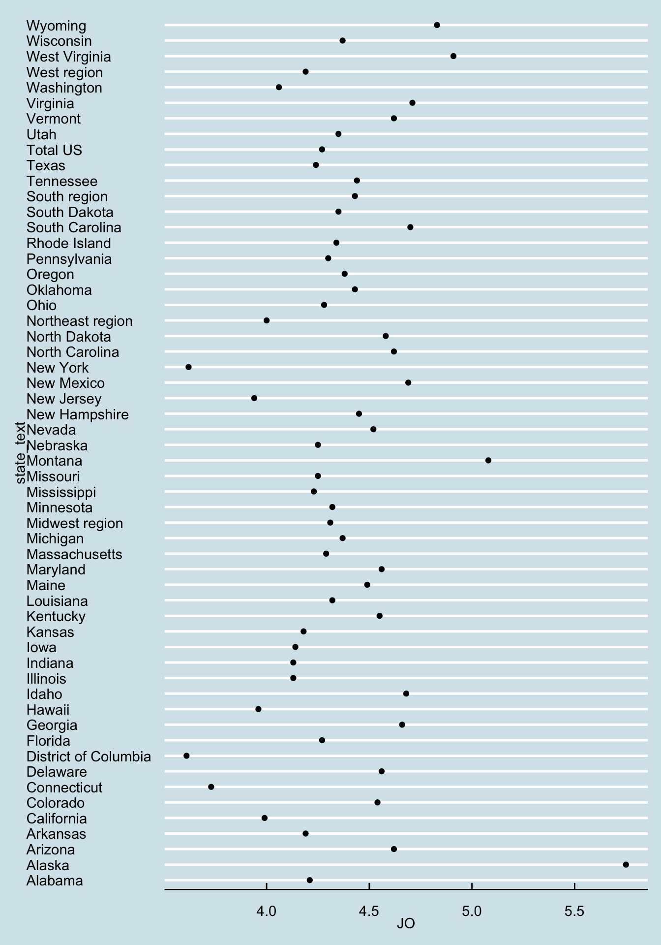
Looks like we should all move to Alaska if we want a job!
5 Snapshotting your environment
You just added a new package to the library, and used it in a script. This means that we should update the lockfile to reflect the new dependency on ggthemes. 6
6 ggplot2 comes with tidyverse, so it should already be in the lockfile.
In the terminal, run
renv::status()and note the discrepency.In the terminal, run
renv::snapshot()and select “yes”.
This will update the lockfile.
- In the terminal, run
renv::status()to make sure everything is up-to-date.
6 Submit to Github
If you haven’t already, commit everything and push to Github!