R Data Wrangling: the tidyverse
Tidy packages in R for data science
February 25, 2026
Packages and Environments in R
What is a package?
A package is
a set of functions
defined outside the current project (usually by someone else).
For R, most packages are hosted on CRAN (Comprehensive R Archive Network), which makes installing packages easy.
You can also easily install packages directly from GitHub.
Packages are incredibly useful and will be a part of any project you work on.
Installing and Loading Packages
The base command for installing packages is
This will download the package from CRAN, and store it on your computer.
Installing and Loading Packages
If you then want to use a function from the package, you have two options:
- Explicit reference for each function
- Loading the whole package
Neither of these options will work if the package isn’t installed!
Package Versions
Packages are functions managed by someone else.
Sometimes those people update the functions.
- Great! Probably the new functions are better!
- But sometimes this is catastrophic for you.
If your code relies entirely on v0.9 of some_function() which always returned a boolean,
and now v1.0 returns an integer,
all of your code using some_function() just broke.
Real World Example of Package Version Issues
dplyr has a function called filter() which is used to filter rows from a data.frame.
Originally, filter_() was an option for standard evaluation, which allowed you to use strings instead of unquoted variable names.
In dplyr v1.0.0, filter_() was removed (and replaced by other methods of standard evaluation).
This change fundamentally broke any code that used filter_(), unless they were preserving their coding environment.
filter_() was first deprecated in v0.7.0, which means it was marked for removal and threw a warning, but still worked. This is a common practice to give users time to update their code.
Environments
Environments will let us be explicit about which package versions we are using.
Allow you to keep track of what packages you use, and their versions.
Load those specific versions of packages at any later date.
This makes environments incredibly important for reproducibility.
R environments: renv
We will be using renv to handle all of our packages.
Environments
Whenever you start a project,
- Install
renv - Initialize the environment
- Install the rest of your packages
Setting up renv
If you have never installed renv before,
Then, we tell renv to start tracking packages for our project.
This is as simple as,
Setting up renv
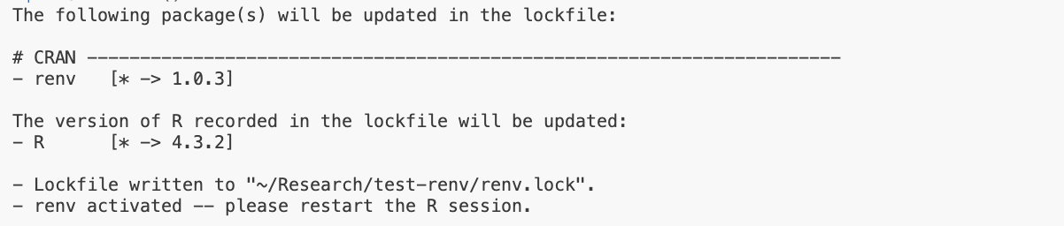
To start with, the only package being tracked is renv itself, and the version of R we are using.
Go ahead and restart the R Session. You should get a new message from renv at the start of the new session.
VS Code can’t find jsonlite, rlang
We also get a warning message at the start of the new session:
VSCode R Session Watcher requires jsonlite, rlang. Please install manually in order to use VSCode-R.Why is this happening?
renv has created an isolated environment for our project.
The only package our system can see is renv itself!
All of the other packages we installed when setting up R and VS Code still exist on our machine, but they cannot be accessed.
Fixing VS Code renv issue
To fix this, we just need to tell renv to install the packages.
If you’ve used renv to install these packages before,
you should see the message “linked from cache”.
renv is smart enough to know it has installed these packages before and instead of redownloading them,
simply provides a link to the right version on our machine.
renv Files
.Rprofile
- This activates
renvat the start of any R session.
renv/
- Where packages for the isolated environment are installed.
renv.lock
- A small file listing packages and their version numbers.
renv Files
renv.lock is the only piece needed to recreate your environment!
So renv/ doesn’t get commited to git, which is good, because it can be large.
Taking Snapshots
Once you start using packages in your project, you need to tell renv to record them.
You do this by taking a snapshot.
This will update the renv.lock file with the packages you have installed and their versions.
Restoring a renv Environment
If you have a renv.lock file, you can restore the environment on any machine.
This is what your collaborators will do when they clone your project, and what you will do when you come back to the project in the future.
The tidyverse
Introducing the tidyverse
The tidyverse is an opinionated collection of R packages designed for data science. All packages share an underlying design philosophy, grammar, and data structures.1
Developed in part by Hadley Wickham (a name we will see again) and supported by the company behind RStudio.
The most popular collection of R packages.
Specifically designed for readable data science.
Installing the tidyverse
Once it is installed for our environment, we can call,
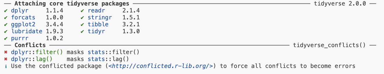
Which prints a nice message showing the packages loaded.
Namespaces
You cannot have two functions with the same name in your environment.
When we load a package, if it conflicts with a function name already in our environment, it will overwrite it to the new function.
You can still use the old function by explicitly calling it with the original package name.
Some tidyverse packages
tibble: A replacement for data.frame object, with better printing
dplyr: Data science functions for adding new columns, filtering data, summarizing, etc.
lubridate: Makes it easier to work with dates.
stringr: Better regular expression and string matching.
readr: Import and export functions (for CSVs)
tibble printing
Shows variable types, dimensions.
Limits printing to not flood console.
tibble list columns
A powerful feature of the tibble type is being able to store any object in a tibble column.
tibble list columns
This means you can have a tibble with
- a column of data sets (nested tibbles)
- a column of fitted models
- a column of model summary stats (R^2, etc.)
dplyr
A set of verbs to work with tibbles.
We will work with a built in dataset: mtcars.
# A tibble: 32 × 11
     mpg   cyl  disp    hp  drat    wt  qsec    vs    am  gear  carb
   <dbl> <dbl> <dbl> <dbl> <dbl> <dbl> <dbl> <dbl> <dbl> <dbl> <dbl>
 1  21       6  160    110  3.9   2.62  16.5     0     1     4     4
 2  21       6  160    110  3.9   2.88  17.0     0     1     4     4
 3  22.8     4  108     93  3.85  2.32  18.6     1     1     4     1
 4  21.4     6  258    110  3.08  3.22  19.4     1     0     3     1
 5  18.7     8  360    175  3.15  3.44  17.0     0     0     3     2
 6  18.1     6  225    105  2.76  3.46  20.2     1     0     3     1
 7  14.3     8  360    245  3.21  3.57  15.8     0     0     3     4
 8  24.4     4  147.    62  3.69  3.19  20       1     0     4     2
 9  22.8     4  141.    95  3.92  3.15  22.9     1     0     4     2
10  19.2     6  168.   123  3.92  3.44  18.3     1     0     4     4
# ℹ 22 more rows
You can see a list of the built in datasets by calling data().
dplyr filter
Filtering datasets allows you to select rows based off of a logical condition.
The first argument is the tibble, the second the condition.
# A tibble: 7 × 11
    mpg   cyl  disp    hp  drat    wt  qsec    vs    am  gear  carb
  <dbl> <dbl> <dbl> <dbl> <dbl> <dbl> <dbl> <dbl> <dbl> <dbl> <dbl>
1  21       6  160    110  3.9   2.62  16.5     0     1     4     4
2  21       6  160    110  3.9   2.88  17.0     0     1     4     4
3  21.4     6  258    110  3.08  3.22  19.4     1     0     3     1
4  18.1     6  225    105  2.76  3.46  20.2     1     0     3     1
5  19.2     6  168.   123  3.92  3.44  18.3     1     0     4     4
6  17.8     6  168.   123  3.92  3.44  18.9     1     0     4     4
7  19.7     6  145    175  3.62  2.77  15.5     0     1     5     6
dplyr filter
You can filter on multiple conditions using the & operator.
Piping
dplyr verbs are designed to be used with a pipe.
A pipe takes the output from the left, and passes it to the first argument on the right.
In R, the pipe operation is: |>
# A tibble: 7 × 11
mpg cyl disp hp drat wt qsec vs am gear carb
<dbl> <dbl> <dbl> <dbl> <dbl> <dbl> <dbl> <dbl> <dbl> <dbl> <dbl>
1 21 6 160 110 3.9 2.62 16.5 0 1 4 4
2 21 6 160 110 3.9 2.88 17.0 0 1 4 4
3 21.4 6 258 110 3.08 3.22 19.4 1 0 3 1
4 18.1 6 225 105 2.76 3.46 20.2 1 0 3 1
5 19.2 6 168. 123 3.92 3.44 18.3 1 0 4 4
6 17.8 6 168. 123 3.92 3.44 18.9 1 0 4 4
7 19.7 6 145 175 3.62 2.77 15.5 0 1 5 6Alternate Pipe
In R, the pipe operation is: |>
You may also see %>% used as a pipe.
This is from the magrittr package, and was used before R had a base pipe. The two are mostly interchangeable.
Does anyone know what painting René Magritte is famous for?
Chaining pipes
# A tibble: 1 × 11
    mpg   cyl  disp    hp  drat    wt  qsec    vs    am  gear  carb
  <dbl> <dbl> <dbl> <dbl> <dbl> <dbl> <dbl> <dbl> <dbl> <dbl> <dbl>
1 19.7 6 145 175 3.62 2.77 15.5 0 1 5 6This is even more readable with a return after each pipe.
dplyr mutate
Possibly the most useful data science verb.
Mutate lets you create new columns in your tibble.
# A tibble: 32 × 12
     mpg   cyl  disp    hp  drat    wt  qsec    vs    am  gear  carb new_col
   <dbl> <dbl> <dbl> <dbl> <dbl> <dbl> <dbl> <dbl> <dbl> <dbl> <dbl>   <dbl>
 1  21       6  160    110  3.9   2.62  16.5     0     1     4     4    78.0
 2  21       6  160    110  3.9   2.88  17.0     0     1     4     4    74.3
 3  22.8     4  108     93  3.85  2.32  18.6     1     1     4     1    56.1
 4  21.4     6  258    110  3.08  3.22  19.4     1     0     3     1    70.2
 5  18.7     8  360    175  3.15  3.44  17.0     0     0     3     2   115.
 6  18.1     6  225    105  2.76  3.46  20.2     1     0     3     1    66.3
 7  14.3     8  360    245  3.21  3.57  15.8     0     0     3     4   133.
 8  24.4     4  147.    62  3.69  3.19  20       1     0     4     2    35.4
 9  22.8     4  141.    95  3.92  3.15  22.9     1     0     4     2    46.2
10  19.2     6  168.   123  3.92  3.44  18.3     1     0     4     4    71.8
# ℹ 22 more rows
dplyr multiple mutates
If you want to do multiple mutates, you can either
- add another mutate function
- add another declaration separated by a comma
dplyr mutate functions
Mutate works with any function that returns a vector of the same length.
# A tibble: 32 × 12
     mpg   cyl  disp    hp  drat    wt  qsec    vs    am  gear  carb cyl_sqrt
   <dbl> <dbl> <dbl> <dbl> <dbl> <dbl> <dbl> <dbl> <dbl> <dbl> <dbl>    <dbl>
 1  21       6  160    110  3.9   2.62  16.5     0     1     4     4     2.45
 2  21       6  160    110  3.9   2.88  17.0     0     1     4     4     2.45
 3  22.8     4  108     93  3.85  2.32  18.6     1     1     4     1     2
 4  21.4     6  258    110  3.08  3.22  19.4     1     0     3     1     2.45
 5  18.7     8  360    175  3.15  3.44  17.0     0     0     3     2     2.83
 6  18.1     6  225    105  2.76  3.46  20.2     1     0     3     1     2.45
 7  14.3     8  360    245  3.21  3.57  15.8     0     0     3     4     2.83
 8  24.4     4  147.    62  3.69  3.19  20       1     0     4     2     2
 9  22.8     4  141.    95  3.92  3.15  22.9     1     0     4     2     2
10  19.2     6  168.   123  3.92  3.44  18.3     1     0     4     4     2.45
# ℹ 22 more rows
This is very useful, as it can work with custom functions you write as well.
dplyr select
select() lets you choose which columns of your data to keep,
- or not to keep, using
-in front of the column name.
dplyr summarize
Summarize lets you collapse your data using functions that take a vector and return a single value.
dplyr summarize
We could summarize multiple columns or operations at once.
dplyr group_by
What if we want summaries for each quantity of cylinders (cyl)?
We could filter the data first, then summarize, and write a loop for each cylinder value…
dplyr main verbs
filter()mutate()select()summarize()group_by()the pipe:
|>
With all of these, you can do most data wrangling!
Other useful dplyr verbs
arrange()sort your data by a column
distinct()keep only unique rows
rename()rename a column
Non-tibble functions
if_else()vectorized if-else, useful within mutates
case_when()use instead of nested if_else statements
lag()andlead()shift values forward or back
Class Activity
Class Activity
- Create a temporary VS Code workspace
- Initialize
renv - Install
tidyverseand load it into an R session - Inspect the built-in dataset
starwars - Use a pipe to filter the dataset for only “Droids”
- Use a pipe and mutate to calculate the BMI (mass / height^2) for each character
- Note: height is given in cm, you’ll need to convert it to meters
Merging
dplyr _join functions
Two example data.frames that we will use:
dplyr::full_join()
Keeps all observations from both the x (left) and y (right) datasets.
dplyr::left_join()
Keeps all observations from the x (left) dataset,
but only the matches from the y (right) dataset.
dplyr::right_join()
Keeps all observations from the y (right) dataset,
but only the matches from the x (left) dataset.
dplyr::inner_join()
Keeps only matches between the two datasets.
dplyr filtering joins
semi_join()
Keep observations in x (left) with a possible match in y (right).
Note: only observations in x are returned, no values from y.
dplyr filtering joins
anti_join()
Keep observations in x (left) without a possible match in y (right).
Note: only observations in x are returned, no values from y.
Merging by different column names
Often you will have slightly different identifying column names between two datasets.
We can handle this using join_by() in the “by” argument.
With the join_by() function you can do inequality, rolling, or overlapping joins (see the documentation).
“tidy” Data
“tidy” Data
- Each variable is a column
- Each observation is a row
This sounds almost tautological.
But a lot of data is not stored this way.
Which of the following tables of stock prices is tidy?
# A tibble: 3 × 3
  stock `2024-01-01` `2024-01-02`
  <chr>        <dbl>        <dbl>
1 A              100          105
2 B               98           95
3 C               99          103
# A tibble: 6 × 3
stock date price
<chr> <date> <dbl>
1 A 2024-01-01 100
2 A 2024-01-02 105
3 B 2024-01-01 98
4 B 2024-01-02 95
5 C 2024-01-01 99
6 C 2024-01-02 103Why tidy?
Imagine we want to add another variable—volume—to the stock price tables.
# A tibble: 6 × 3
  stock   `2024-01-01` `2024-01-02`
  <chr>          <dbl>        <dbl>
1 A_price          100          105
2 B_price           98           95
3 C_price           99          103
4 A_vol             50           70
5 B_vol             30           55
6 C_vol             23           60
# A tibble: 6 × 4
stock date price volume
<chr> <date> <dbl> <dbl>
1 A 2024-01-01 100 50
2 A 2024-01-02 105 70
3 B 2024-01-01 98 30
4 B 2024-01-02 95 55
5 C 2024-01-01 99 23
6 C 2024-01-02 103 60This is very easy for tidy data.
But it is hard for nontidy data.
- Do we add a “_price” and “_vol” to each stock row?
- Or to each date column?
- Or store them as two tables?
Making everything tidy
The tidyverse obviously has strong support for tidy data.
In particular, the package tidyr.
We will cover two crucial functions:
tidyr::pivot_longer()tidyr::pivot_wider()
pivot_longer
Pivot functions let you transform a data.frame between wide and long formats.
Let’s look at the stock price data from earlier.
pivot_longer
# A tibble: 3 × 3
  stock `2024-01-01` `2024-01-02`
  <chr>        <dbl>        <dbl>
1 A              100          105
2 B               98           95
3 C 99 103pivot_longer
# A tibble: 3 × 3
  stock `2024-01-01` `2024-01-02`
  <chr>        <dbl>        <dbl>
1 A              100          105
2 B               98           95
3 C               99          103
Instead, we could list the columns not to lengthen.
pivot_longer names
pivot_longer defaults to naming new columns “name” and “value”, but you can override these.
pivot_longer data types
We should also convert the date column to the date-type.
pivot_wider
Sometimes, data can be non-tidy because it is too long.
# A tibble: 8 × 4
  stock date       variable  value
  <chr> <date>     <chr>     <dbl>
1 A     2024-01-01 price       100
2 A     2024-01-01 vol      100000
3 A     2024-01-02 price       105
4 A     2024-01-02 vol      130000
5 B     2024-01-01 price        98
6 B     2024-01-01 vol      120000
7 B     2024-01-02 price        95
8 B     2024-01-02 vol      150000
# A tibble: 4 × 4
stock date price vol
<chr> <date> <dbl> <dbl>
1 A 2024-01-01 100 100000
2 A 2024-01-02 105 120000
3 B 2024-01-01 98 130000
4 B 2024-01-02 95 150000pivot_wider
The two key arguments: names_from = and values_from =.
Why is too long non-tidy?
Imagine we had a variable with a different data type, like a variable for whether the stock price went up or down.
# A tibble: 12 × 4
stock date variable value
<chr> <date> <chr> <chr>
1 A 2024-01-01 price 100
2 A 2024-01-01 vol 1e+05
3 A 2024-01-01 up up
4 A 2024-01-02 price 105
5 A 2024-01-02 vol 130000
6 A 2024-01-02 up down
7 B 2024-01-01 price 98
8 B 2024-01-01 vol 120000
9 B 2024-01-01 up up
10 B 2024-01-02 price 95
11 B 2024-01-02 vol 150000
12 B 2024-01-02 up down Notice that the value column is now a character, as this is the most general data type that can accomodate all of the values.
Column Patterns in Pivoting
Using names_sep argument, we can split a column into multiple columns based on a pattern.
# A tibble: 2 × 7
date A_price B_price C_price A_vol B_vol C_vol
<date> <dbl> <dbl> <dbl> <dbl> <dbl> <dbl>
1 2024-01-01 100 98 99 50 30 23
2 2024-01-02 105 95 103 70 55 60# A tibble: 12 × 4
date stock variable value
<date> <chr> <chr> <dbl>
1 2024-01-01 A price 100
2 2024-01-01 B price 98
3 2024-01-01 C price 99
4 2024-01-01 A vol 50
5 2024-01-01 B vol 30
6 2024-01-01 C vol 23
7 2024-01-02 A price 105
8 2024-01-02 B price 95
9 2024-01-02 C price 103
10 2024-01-02 A vol 70
11 2024-01-02 B vol 55
12 2024-01-02 C vol 60Column Patterns in Pivoting
You can also use names_sep in pivot_wider to combine multiple columns into one.
# A tibble: 4 × 4
  stock date       price    vol
  <chr> <date>     <dbl>  <dbl>
1 A     2024-01-01   100 100000
2 A     2024-01-02   105 120000
3 B     2024-01-01    98 130000
4 B 2024-01-02 95 150000# A tibble: 2 × 5
date price_A price_B vol_A vol_B
<date> <dbl> <dbl> <dbl> <dbl>
1 2024-01-01 100 98 100000 130000
2 2024-01-02 105 95 120000 150000Obviously, this is now non-tidy data.
Pivoting
With
pivot_longerpivot_wider
it’s easy to convert from long to wide data formats.
With these tools, you can “tidy” most any dataset.
Once data is tidy it’s easy to lengthen or widen the data for any calculations.
Common Examples of non-tidy data
Column headers are values, not variable names.
Multiple variables are stored in one column.
Variables are stored in both rows and columns.
Multiple types of observational units are stored in the same table.
A single observational unit is stored in multiple tables.
from Tidy Data
Live Coding Example
Live Coding Example
- Example of tidying a dataset:
data("world_bank_pop")fromtidyrpackage - Using
pivot_longerandpivot_wider