R Functions & Regressions

A functional approach to programming

Matthew DeHaven

March 18, 2026

Functions

Functions…

take input(s)
do something
return an ouput

R is a Functional Language

R, at its heart, is a functional programming (FP) language. This means that it provides many tools for the creation and manipulation of functions. In particular, R has what’s known as first class functions. You can do anything with functions that you can do with vectors: you can assign them to variables, store them in lists, pass them as arguments to other functions, create them inside functions, and even return them as the result of a function. Hadley Wickham, Advanced R

Why use functions?

Functions make your code:

more flexible
less repetitive
more readable (potentially)

A Basic Function

Here is a basic, if not exciting, function:

cube <- function(input) {
  cubed <- input ^ 3        
  return(cubed)             
}
cube(2)

[1] 8

Take inputs
Do something
Return output

Syntax

Functions are always declared using the function function(),

followed by curly braces { } which demark what the function actually does.

Most functions will end with a return() call, though this is not strictly required.

“Degenerate” functions

myfunc1 <- function() {print("Just prints something")}
myfunc1()

[1] "Just prints something"

Which is just to show that technically inputs and outputs are not necessary.

In fact, we could make a function that does nothing…not very useful.

myfunc2 <- function() { }
myfunc2()

NULL

Variable Scope

Functions have their own “environment” for variables.

cubed <- "Outside function"
cube <- function(x) {
  cubed <- x ^ 3
  return(cubed)
}
cubed

[1] "Outside function"

Even if we call our function, the value for cubed is not overwritten in our R session environment.

cube(3)

[1] 27

cubed

[1] "Outside function"

Breaking Function Scope

<<- breaks the scope of a function and affects vaiables outside

cubed <- "Outside function"
cube <- function(x) {
  cubed <<- x ^ 3
  return(cubed)
}
cube(3)

[1] 27

cubed

[1] 27

But this is a really bad idea.

You should only allow functions to affect your session by returning values.

Otherwise, it is very confusing to tell what is changing a variable.

Limiting Function Scope

Technically, you can use a variable defined outside a function inside a function.

beta <- 0.99
utility <- function(x) {
  u <- beta * log(x)
  return(u)
}
utility(10)

[1] 2.279559

But this is also a bad idea.

Functions are meant to be flexible and portable
By relying on a session variable we’ve made this function dependent on the current setting.

Adding Additional Arguments

Instead, we should pass beta as an additional argument for our function.

utility <- function(x, beta) {
  u <- beta * log(x)
  return(u)
}

Now we can call our function by passing two values.

utility(10, 0.99)

[1] 2.279559

This makes our function more general, flexible, and reusable.

Setting a Default Argument

When declaring a function, you can set a default value for an argument.

utility <- function(x, beta = 0.99) {
  u <- beta * log(x)
  return(u)
}
utility(10)

[1] 2.279559

That default value will be used unless you specify a new value to overwrite it.

utility(10, beta = 0.78)

[1] 1.796016

Ordering of Arguments

Functions assume unlabelled arguments are given in the order they were declared.

i.e. the first argument is our consumption value, and the second is our beta.

utility(10, 0.98)

[1] 2.256533

You can always be explicit about function arguments as well.

utility(x = 10, beta = 0.98)

[1] 2.256533

And if you are explicit, you can change the order of arguments.

utility(beta = 0.99, x = 10)

[1] 2.279559

CRRA Utility

Let’s declare a CRRA utility function,

\[ U(C) = \beta \frac{C^{1-\gamma}}{1-\gamma} \]

In our code, this looks like

utility <- function(x, gamma, beta = 0.99) {
  u <- beta * (x ^ (1 - gamma)) / (1 - gamma)
  return(u)
}
utility(10, gamma = 0.5)

[1] 6.26131

CRRA Utility

Let’s declare a CRRA utility function,

\[ U(C) = \beta \frac{C^{1-\gamma}}{1-\gamma} \]

What happens if we run when gamma = 1?

utility(10, gamma = 1)

[1] Inf

If you paid attention in Macro, then you know that CRRA utility with $\gamma \rightarrow 1$ converges to log utility.

If-Else Statements within Functions

We can implement this with an if-else statement within our function.

utility <- function(x, gamma, beta = 0.99) {
  if (gamma == 1) {
    u <- beta * log(x)
  } else {
    u <- beta * (x ^ (1 - gamma)) / (1 - gamma)
  }
  return(u)
}

Now our function works in both cases:

utility(10, gamma = 0.5)

[1] 6.26131

utility(10, gamma = 1)

[1] 2.279559

Printing out a function

We can always inspect the actual code for a function by calling it without the parentheses ().

cube

function (x) 
{
    cubed <<- x^3
    return(cubed)
}

Printing out a function

This works for functions from other packages too.

dplyr::lag

function (x, n = 1L, default = NULL, order_by = NULL, ...) 
{
    if (inherits(x, "ts")) {
        abort("`x` must be a vector, not a <ts>, do you want `stats::lag()`?")
    }
    check_dots_empty0(...)
    check_number_whole(n)
    if (n < 0L) {
        abort("`n` must be positive.")
    }
    shift(x, n = n, default = default, order_by = order_by)
}
<bytecode: 0x10a27c250>
<environment: namespace:dplyr>

Anonymous Functions

Anonymous functions are functions that do not have a name.

Anonymous Functions

Anonymous functions are functions that do not have a name.

This means they are not stored as a variable that you can use over again, but exist only for a moment.

function(x) {x ^ 3}

function (x) 
{
    x^3
}

For functions that only take one line, you can drop the curly brackets.

function(x) x ^ 3

function (x) 
x^3

When would we use this?

`purrr::map()` family

Map Family of Functions

We saw briefly the *apply() family of base R functions (when we were looking at loops).

The map() family is the tidyverse equivalent and are nicer to use.

library(purrr)
some_vector <- c(1, 4, 6)
map(some_vector, cube)

[[1]]
[1] 1

[[2]]
[1] 64

[[3]]
[1] 216

Map Function

The map() function always

takes a vector (or list) for input
calls a function on each element
returns a list as the result

map(list(1, 4, 6), cube)

[[1]]
[1] 1

[[2]]
[1] 64

[[3]]
[1] 216

Using an Anonymous Function with `map()`

This is an example where we may want to declare an anonymous function.

map(1:3, function(x) {x ^ 3 + 2})

[[1]]
[1] 3

[[2]]
[1] 10

[[3]]
[1] 29

Using an Anonymous Function with `map()`

And again, because our function is only one line, we could drop the curly braces.

map(1:3, function(x) x ^ 3 + 2)

[[1]]
[1] 3

[[2]]
[1] 10

[[3]]
[1] 29

Multiline Anonymous Functions

Conversely, you could have a multiline anonymous function.

datasets <- list(mtcars, iris)
map(datasets, function(x) {
  x |>
    dplyr::select(1:3) |>
    summary()
})

[[1]]
      mpg             cyl             disp      
 Min.   :10.40   Min.   :4.000   Min.   : 71.1  
 1st Qu.:15.43   1st Qu.:4.000   1st Qu.:120.8  
 Median :19.20   Median :6.000   Median :196.3  
 Mean   :20.09   Mean   :6.188   Mean   :230.7  
 3rd Qu.:22.80   3rd Qu.:8.000   3rd Qu.:326.0  
 Max.   :33.90   Max.   :8.000   Max.   :472.0  

[[2]]
  Sepal.Length    Sepal.Width     Petal.Length  
 Min.   :4.300   Min.   :2.000   Min.   :1.000  
 1st Qu.:5.100   1st Qu.:2.800   1st Qu.:1.600  
 Median :5.800   Median :3.000   Median :4.350  
 Mean   :5.843   Mean   :3.057   Mean   :3.758  
 3rd Qu.:6.400   3rd Qu.:3.300   3rd Qu.:5.100  
 Max.   :7.900   Max.   :4.400   Max.   :6.900

`map` Return Types

By default, map() will always return a list.

It does not know the datatype of the objects you are returning,

and a list works with any data type and with a mix of data types.

If you do know your datatype, you could use…

map_lgl()
map_int()
map_dbl()
map_chr()

Which will all return a vector of that data type.

Example with `map_dbl()`

Using our prior map example,

map_dbl(1:3, function(x) x ^ 3 + 2)

[1]  3 10 29

If we use the wrong one, however, we get an error.

map_lgl(1:3, function(x) x ^ 3 + 2)

Error in `map_lgl()`:
ℹ In index: 1.
Caused by error:
! Can't coerce from a number to a logical.

Example with `fredr` package

We saw before that map() was convenient for working with fredr package.

library(fredr)
c("UNRATE", "GDP", "FEDFUNDS") |>
  map(fredr) |>
 list_rbind()

This map function returns data.frames (tibbles) and then list_rbind combines them by rbind-ing them.

rbind() takes two data.frames and stacks them on top of each other
cbind() takes two data.frames and stacks them beside one another

Regression Functions

Regressions

The workhorse of economics research is linear regression.

The simplest form of which is, \[ Y = \beta X + \epsilon \]

Given a set of values for $Y$ and $X$, we can estimate $\hat{\beta}$.

Generating some example data

library(tidyverse)
set.seed(42) ## Makes random draws reproducible
tb <- tibble(
  x = sample(1:10, 100, replace = TRUE) + rnorm(100),
  y = 5 * x + 20 * rnorm(100)
  )
tb |> ggplot(aes(x = x, y = y)) + geom_point()

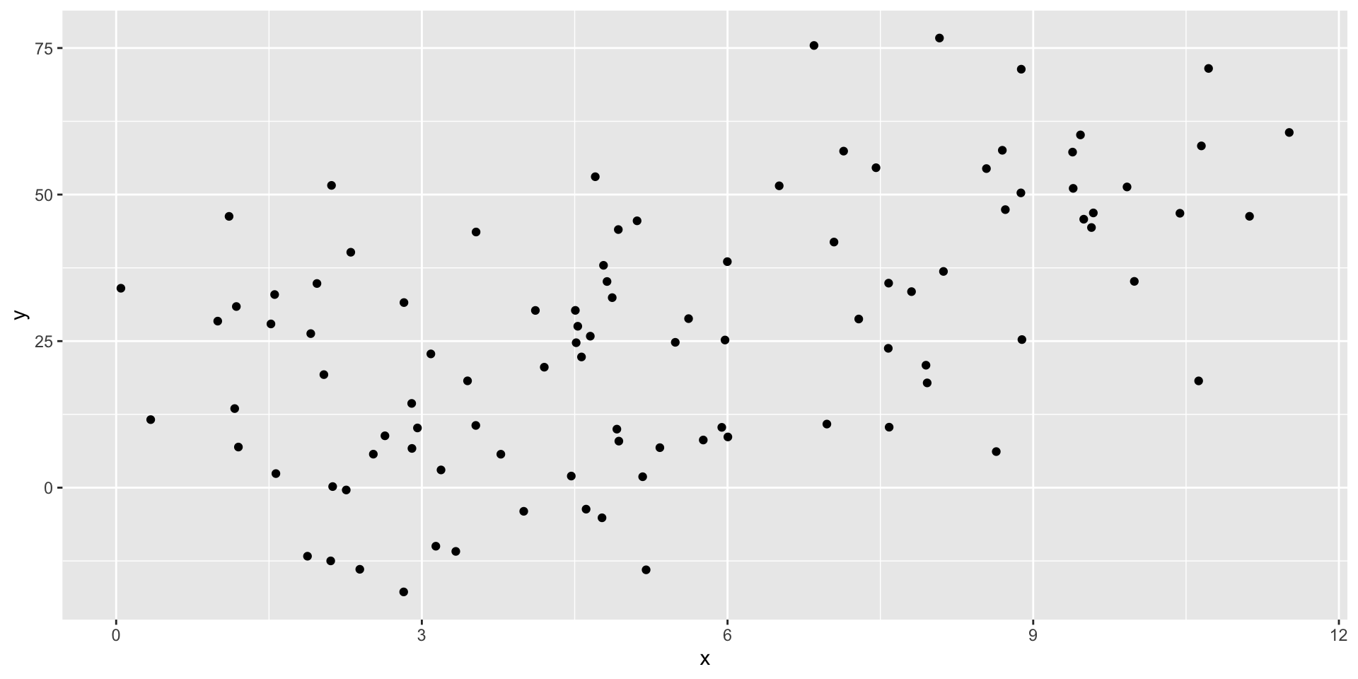
Estimating $\beta$

R has a built in function for linear models: lm().

m <- lm("y ~ x", data = tb)
m


Call:
lm(formula = "y ~ x", data = tb)

Coefficients:
(Intercept)            x  
      4.633        4.100

Printing the model returns only a few pieces of information, but there’s much more stored within.

`summary()` for detailed information

summary(m)


Call:
lm(formula = "y ~ x", data = tb)

Residuals:
    Min      1Q  Median      3Q     Max 
-39.971 -14.708  -0.024  13.895  42.721 

Coefficients:
            Estimate Std. Error t value Pr(>|t|)    
(Intercept)    4.633      3.939   1.176    0.242    
x              4.100      0.643   6.377 5.97e-09 ***
---
Signif. codes:  0 '***' 0.001 '**' 0.01 '*' 0.05 '.' 0.1 ' ' 1

Residual standard error: 18.85 on 98 degrees of freedom
Multiple R-squared:  0.2932,    Adjusted R-squared:  0.286 
F-statistic: 40.66 on 1 and 98 DF,  p-value: 5.973e-09

Structure of `lm()` models

str(m)

List of 12
 $ coefficients : Named num [1:2] 4.63 4.1
  ..- attr(*, "names")= chr [1:2] "(Intercept)" "x"
 $ residuals    : Named num [1:100] 26.09 -19.69 6.29 5.99 22.93 ...
  ..- attr(*, "names")= chr [1:100] "1" "2" "3" "4" ...
 $ effects      : Named num [1:100] -266.88 -120.21 1.64 7.22 24.75 ...
  ..- attr(*, "names")= chr [1:100] "(Intercept)" "x" "" "" ...
 $ rank         : int 2
 $ fitted.values: Named num [1:100] 14.1 26.5 13 45.3 48.6 ...
  ..- attr(*, "names")= chr [1:100] "1" "2" "3" "4" ...
 $ assign       : int [1:2] 0 1
 $ qr           :List of 5
  ..$ qr   : num [1:100, 1:2] -10 0.1 0.1 0.1 0.1 0.1 0.1 0.1 0.1 0.1 ...
  .. ..- attr(*, "dimnames")=List of 2
  .. .. ..$ : chr [1:100] "1" "2" "3" "4" ...
  .. .. ..$ : chr [1:2] "(Intercept)" "x"
  .. ..- attr(*, "assign")= int [1:2] 0 1
  ..$ qraux: num [1:2] 1.1 1.01
  ..$ pivot: int [1:2] 1 2
  ..$ tol  : num 1e-07
  ..$ rank : int 2
  ..- attr(*, "class")= chr "qr"
 $ df.residual  : int 98
 $ xlevels      : Named list()
 $ call         : language lm(formula = "y ~ x", data = tb)
 $ terms        :Classes 'terms', 'formula'  language y ~ x
  .. ..- attr(*, "variables")= language list(y, x)
  .. ..- attr(*, "factors")= int [1:2, 1] 0 1
  .. .. ..- attr(*, "dimnames")=List of 2
  .. .. .. ..$ : chr [1:2] "y" "x"
  .. .. .. ..$ : chr "x"
  .. ..- attr(*, "term.labels")= chr "x"
  .. ..- attr(*, "order")= int 1
  .. ..- attr(*, "intercept")= int 1
  .. ..- attr(*, "response")= int 1
  .. ..- attr(*, ".Environment")=<environment: 0x13d181e98> 
  .. ..- attr(*, "predvars")= language list(y, x)
  .. ..- attr(*, "dataClasses")= Named chr [1:2] "numeric" "numeric"
  .. .. ..- attr(*, "names")= chr [1:2] "y" "x"
 $ model        :'data.frame':  100 obs. of  2 variables:
  ..$ y: num [1:100] 40.16 6.83 19.29 51.3 71.52 ...
  ..$ x: num [1:100] 2.3 5.34 2.04 9.92 10.72 ...
  ..- attr(*, "terms")=Classes 'terms', 'formula'  language y ~ x
  .. .. ..- attr(*, "variables")= language list(y, x)
  .. .. ..- attr(*, "factors")= int [1:2, 1] 0 1
  .. .. .. ..- attr(*, "dimnames")=List of 2
  .. .. .. .. ..$ : chr [1:2] "y" "x"
  .. .. .. .. ..$ : chr "x"
  .. .. ..- attr(*, "term.labels")= chr "x"
  .. .. ..- attr(*, "order")= int 1
  .. .. ..- attr(*, "intercept")= int 1
  .. .. ..- attr(*, "response")= int 1
  .. .. ..- attr(*, ".Environment")=<environment: 0x13d181e98> 
  .. .. ..- attr(*, "predvars")= language list(y, x)
  .. .. ..- attr(*, "dataClasses")= Named chr [1:2] "numeric" "numeric"
  .. .. .. ..- attr(*, "names")= chr [1:2] "y" "x"
 - attr(*, "class")= chr "lm"

It’s just a big list!

You can access certain components (ex. m$residuals).

Summary also returns a list

m |> summary() |> str()

List of 11
 $ call         : language lm(formula = "y ~ x", data = tb)
 $ terms        :Classes 'terms', 'formula'  language y ~ x
  .. ..- attr(*, "variables")= language list(y, x)
  .. ..- attr(*, "factors")= int [1:2, 1] 0 1
  .. .. ..- attr(*, "dimnames")=List of 2
  .. .. .. ..$ : chr [1:2] "y" "x"
  .. .. .. ..$ : chr "x"
  .. ..- attr(*, "term.labels")= chr "x"
  .. ..- attr(*, "order")= int 1
  .. ..- attr(*, "intercept")= int 1
  .. ..- attr(*, "response")= int 1
  .. ..- attr(*, ".Environment")=<environment: 0x13d181e98> 
  .. ..- attr(*, "predvars")= language list(y, x)
  .. ..- attr(*, "dataClasses")= Named chr [1:2] "numeric" "numeric"
  .. .. ..- attr(*, "names")= chr [1:2] "y" "x"
 $ residuals    : Named num [1:100] 26.09 -19.69 6.29 5.99 22.93 ...
  ..- attr(*, "names")= chr [1:100] "1" "2" "3" "4" ...
 $ coefficients : num [1:2, 1:4] 4.633 4.1 3.939 0.643 1.176 ...
  ..- attr(*, "dimnames")=List of 2
  .. ..$ : chr [1:2] "(Intercept)" "x"
  .. ..$ : chr [1:4] "Estimate" "Std. Error" "t value" "Pr(>|t|)"
 $ aliased      : Named logi [1:2] FALSE FALSE
  ..- attr(*, "names")= chr [1:2] "(Intercept)" "x"
 $ sigma        : num 18.9
 $ df           : int [1:3] 2 98 2
 $ r.squared    : num 0.293
 $ adj.r.squared: num 0.286
 $ fstatistic   : Named num [1:3] 40.7 1 98
  ..- attr(*, "names")= chr [1:3] "value" "numdf" "dendf"
 $ cov.unscaled : num [1:2, 1:2] 0.04366 -0.00626 -0.00626 0.00116
  ..- attr(*, "dimnames")=List of 2
  .. ..$ : chr [1:2] "(Intercept)" "x"
  .. ..$ : chr [1:2] "(Intercept)" "x"
 - attr(*, "class")= chr "summary.lm"

It can be useful to access specific components with summary(m)$coefficients.

Tidying model results

broom is a package that tries to “tidy” model results into data.frames.

renv::install("broom")

Let’s see what it does for our little model:

broom::tidy(m)

# A tibble: 2 × 5
  term        estimate std.error statistic       p.value
  <chr>          <dbl>     <dbl>     <dbl>         <dbl>
1 (Intercept)     4.63     3.94       1.18 0.242        
2 x               4.10     0.643      6.38 0.00000000597

Much easier to work with!

broom is written to create standardized results from many different models from many different packages.

Subsets of data

First, we are going to add some random groups to our data.

tb <- tb |>
  mutate(group = sample(c("A", "B", "C"), 100, replace = TRUE))
tb |> ggplot(aes(x = x, y = y, color = group)) + geom_point()

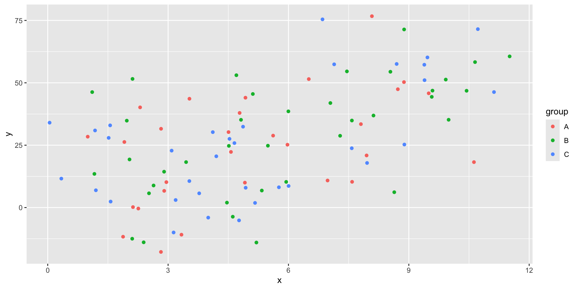
Nesting tibbles

What if we want to run multiple regressions, one on each group?

One option would be filter the data, then call lm three times.

Or we can set up nested tibbles.

ntb <- tb |>
  nest(data = c(x, y))
ntb

# A tibble: 3 × 2
  group data             
  <chr> <list>           
1 A     <tibble [29 × 2]>
2 B     <tibble [37 × 2]>
3 C     <tibble [34 × 2]>

We’ve separated our data into three tibbles, each stored as a row in our parent tibble.

Running `lm` on nested tibbles

Now we can use this nested format to run all three of our models at once.

ntb |>
  mutate(model = map(data, function(tb) lm("y ~ x", data = tb) ))

# A tibble: 3 × 3
  group data              model 
  <chr> <list>            <list>
1 A     <tibble [29 × 2]> <lm>  
2 B     <tibble [37 × 2]> <lm>  
3 C     <tibble [34 × 2]> <lm>

Now we have a column of lm models!

Tidying nested model results

Now we can tidy those models so we can contrast all of the results.

stb <- ntb |>
  mutate(model = map(data, function(tb) lm("y ~ x", data = tb) )) |>
  mutate(summary = map(model, broom::tidy))
stb

# A tibble: 3 × 4
  group data              model  summary         
  <chr> <list>            <list> <list>          
1 A     <tibble [29 × 2]> <lm>   <tibble [2 × 5]>
2 B     <tibble [37 × 2]> <lm>   <tibble [2 × 5]>
3 C     <tibble [34 × 2]> <lm>   <tibble [2 × 5]>

We have all of the model summaries now, but we need to unnest the tibble to easily compare them.

Unnesting a tibble

stb |>
  unnest(summary) |>
  select(-c("data", "model")) |>  ## dropping columns to fit on slide
  arrange(term)

# A tibble: 6 × 6
  group term        estimate std.error statistic  p.value
  <chr> <chr>          <dbl>     <dbl>     <dbl>    <dbl>
1 A     (Intercept)     5.42      7.90     0.686 0.499   
2 B     (Intercept)     5.33      6.92     0.770 0.447   
3 C     (Intercept)     3.88      6.36     0.609 0.547   
4 A     x               3.74      1.38     2.72  0.0113  
5 B     x               4.10      1.05     3.89  0.000432
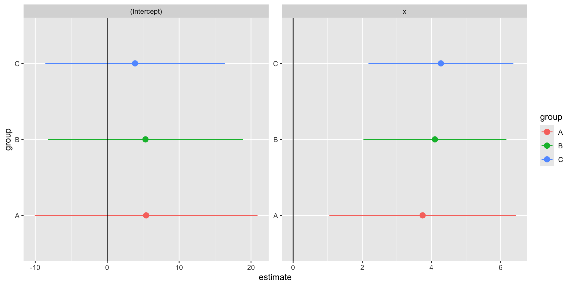
6 C     x               4.27      1.07     4.00  0.000354

We can now easily compare our three models’ $\beta$ estimate for $x$.

Making a coefficient chart

stb |>
  unnest(summary) |>
  ggplot() + 
  geom_point(aes(
    x = estimate,
    y = group,
    color = group
  ),
    size = 3
  ) +
  geom_segment(aes(
    x = estimate - 1.96 * std.error,
    xend = estimate + 1.96 * std.error,
    y = group,
    yend = group,
    color = group
  )) +
  geom_vline(xintercept = 0) +
  facet_wrap(vars(term), scales = "free")

Making a coefficient chart

Nesting Summary

Pros

A clean way to estimate multiple models
Makes full use of tidyverse functions
Easy to add more models, different subsets

Cons

Duplicates data for each row
- This can be very costly for large datasets

Robust Standard Errors

As you know from econometrics class, you shold pretty much always use robust standard errors when you report results.

There are a couple of packages which support this in R,

sandwich

estimatr

We are going to use estimatr today.

renv::install("estimatr")

Robust SE with `estimatr`

library(estimatr)

The package is written to match the syntax of lm().

m  <- lm(y ~ x, data = tb)
mr <- lm_robust(y ~ x, data = tb)

Same point estimates, slightly different standard errors.

tidy(m)

# A tibble: 2 × 5
  term        estimate std.error statistic       p.value
  <chr>          <dbl>     <dbl>     <dbl>         <dbl>
1 (Intercept)     4.63     3.94       1.18 0.242        
2 x               4.10     0.643      6.38 0.00000000597

tidy(mr)

         term estimate std.error statistic      p.value  conf.low conf.high df
1 (Intercept) 4.633091 4.0673715  1.139087 2.574435e-01 -3.438476  12.70466 98
2           x 4.100106 0.6251976  6.558096 2.574586e-09  2.859422   5.34079 98
  outcome
1       y
2       y

Changing the SE type

estimatr defaults to using “HC2” robust standard errors.

There are options for “HC0”, “HC1”, and “HC3”.

mr <- lm_robust(y ~ x, data = tb, se_type = "HC1")

I can’t really tell you the importance of the small differences between these robust options. You can read more about the math for each here.

If you want to match exactly the robust SEs reported in STATA, use “HC1” or “stata”

mr <- lm_robust(y ~ x, data = tb, se_type = "stata")

Panel Regressions

Fixed effects
Clustering

We will use the fixest package

renv::install("fixest")

library(fixest)

Panel data

Panel data has at least two dimensions

time
groups
- countries, states, people

This is in contrast to time series (just a time dimension) and cross-sectional data.

Example Panel Data

We are going to use the package gapminder to get our example panel data.

renv::install("gapminder")

library(gapminder)
gapminder <- gapminder |> mutate(pop = pop / 1e6, gdpPercap = gdpPercap / 1e3)
gapminder

# A tibble: 1,704 × 6
   country     continent  year lifeExp   pop gdpPercap
   <fct>       <fct>     <int>   <dbl> <dbl>     <dbl>
 1 Afghanistan Asia       1952    28.8  8.43     0.779
 2 Afghanistan Asia       1957    30.3  9.24     0.821
 3 Afghanistan Asia       1962    32.0 10.3      0.853
 4 Afghanistan Asia       1967    34.0 11.5      0.836
 5 Afghanistan Asia       1972    36.1 13.1      0.740
 6 Afghanistan Asia       1977    38.4 14.9      0.786
 7 Afghanistan Asia       1982    39.9 12.9      0.978
 8 Afghanistan Asia       1987    40.8 13.9      0.852
 9 Afghanistan Asia       1992    41.7 16.3      0.649
10 Afghanistan Asia       1997    41.8 22.2      0.635
# ℹ 1,694 more rows

Running OLS with `fixest`

Let’s predict life expectancy using GDP per capita.

mf <- feols(lifeExp ~ gdpPercap, data = gapminder)
summary(mf)

OLS estimation, Dep. Var.: lifeExp
Observations: 1,704
Standard-errors: IID 
             Estimate Std. Error  t value  Pr(>|t|)    
(Intercept) 53.955561   0.314995 171.2902 < 2.2e-16 ***
gdpPercap    0.764883   0.025790  29.6577 < 2.2e-16 ***
---
Signif. codes:  0 '***' 0.001 '**' 0.01 '*' 0.05 '.' 0.1 ' ' 1
RMSE: 10.5   Adj. R2: 0.340326

We could easily have estimated this with

lm() or
lm_robust()

Adding in fixed effects

Let’s add fixed effects for each continent.

mf <- feols(lifeExp ~ gdpPercap | continent, data = gapminder)
summary(mf)

OLS estimation, Dep. Var.: lifeExp
Observations: 1,704
Fixed-effects: continent: 5
Standard-errors: IID 
          Estimate Std. Error t value  Pr(>|t|)    
gdpPercap  0.44527   0.023498 18.9493 < 2.2e-16 ***
---
Signif. codes:  0 '***' 0.001 '**' 0.01 '*' 0.05 '.' 0.1 ' ' 1
RMSE: 8.37531     Adj. R2: 0.578106
                Within R2: 0.174557

Super easy to run!

Notice that it automatically clustered our standard errors to “continent” as well. What if we don’t want that? When Should You Adjust Standard Errors for Clustering (Abadie, Athey, Imbens, Woolridge 2017)

Setting iid standard errors

We can be explicit about standard errors using the “vcov=” argument.

mfiid <- feols(lifeExp ~ gdpPercap | continent, vcov = "iid", data = gapminder)
summary(mfiid)

OLS estimation, Dep. Var.: lifeExp
Observations: 1,704
Fixed-effects: continent: 5
Standard-errors: IID 
          Estimate Std. Error t value  Pr(>|t|)    
gdpPercap  0.44527   0.023498 18.9493 < 2.2e-16 ***
---
Signif. codes:  0 '***' 0.001 '**' 0.01 '*' 0.05 '.' 0.1 ' ' 1
RMSE: 8.37531     Adj. R2: 0.578106
                Within R2: 0.174557

Setting iid standard errors

We can also have clustered standard errors without including fixed effects.

mfc <- feols(lifeExp ~ gdpPercap, cluster = ~ continent, data = gapminder)
summary(mfc)

OLS estimation, Dep. Var.: lifeExp
Observations: 1,704
Standard-errors: Clustered (continent) 
             Estimate Std. Error  t value   Pr(>|t|)    
(Intercept) 53.955561   4.586864 11.76306 0.00029883 ***
gdpPercap    0.764883   0.290197  2.63574 0.05783770 .  
---
Signif. codes:  0 '***' 0.001 '**' 0.01 '*' 0.05 '.' 0.1 ' ' 1
RMSE: 10.5   Adj. R2: 0.340326

Adding another variable

I want to add another fixed effect, so I’m going to add a new column for countries with big vs. small populations.

gapminder <- gapminder |> 
  mutate(big_small = ifelse(pop >= median(pop), "big", "small"))

Running multiple fixed effects

We can add multiple fixed effects with the same syntax as adding more regressors.

mf2fe <- feols(lifeExp ~ gdpPercap | continent + big_small, data = gapminder)
summary(mf2fe)

OLS estimation, Dep. Var.: lifeExp
Observations: 1,704
Fixed-effects: continent: 5,  big_small: 2
Standard-errors: IID 
          Estimate Std. Error t value  Pr(>|t|)    
gdpPercap 0.453664   0.023429  19.363 < 2.2e-16 ***
---
Signif. codes:  0 '***' 0.001 '**' 0.01 '*' 0.05 '.' 0.1 ' ' 1
RMSE: 8.32322     Adj. R2: 0.583092
                Within R2: 0.180956

Comparing models

fixest has a nice function to print multiple models:

etable(mf, mfiid, mf2fe)

                                mf              mfiid              mf2fe
Dependent Var.:            lifeExp            lifeExp            lifeExp
                                                                        
gdpPercap       0.4453*** (0.0235) 0.4453*** (0.0235) 0.4537*** (0.0234)
Fixed-Effects:  ------------------ ------------------ ------------------
continent                      Yes                Yes                Yes
big_small                       No                 No                Yes
_______________ __________________ __________________ __________________
S.E. type                      IID                IID                IID
Observations                 1,704              1,704              1,704
R2                         0.57934            0.57934            0.58456
Within R2                  0.17456            0.17456            0.18096
---
Signif. codes: 0 '***' 0.001 '**' 0.01 '*' 0.05 '.' 0.1 ' ' 1

Speed Comparison: `fixest` and Stata’s `reghdfe`

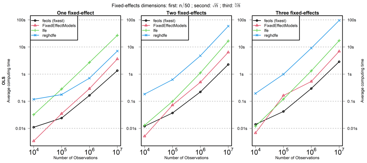
lfe is another R package, reghdfe is a Stata package, and FixedEffectModels is a Julia package.

Source: fixest documentation (comparison run in 2020)

Parallel Processing

Sequential processing (default) is when code is run on one “core”.

Parallel Processing

Parallel processing splits operations over multiple “cores”.

A Slow Function

Imagine we had some slow code that we wanted to run multiple times.

slow_cube <- function(x) {
  Sys.sleep(2)  ## Tells R to wait 2 seconds
  return(x ^ 3)
}

Aside: Measuring Code Speed in R

We will use the package tictoc to measure the time it takes to run our function.

library(tictoc)
tic()
Sys.sleep(1)
toc()

1.006 sec elapsed

If you want more systematic code profiling, you can use the profvis or microbenchmark packages.

Timing our Slow Function

Now we can see how long our slow function takes to run.

tic()
slow_cube(10)

[1] 1000

toc()

2.007 sec elapsed

Timing our Slow Function

And if we ran it multiple times…

tic()
map(1:3, slow_cube)

[[1]]
[1] 1

[[2]]
[1] 8

[[3]]
[1] 27

toc()

6.016 sec elapsed

Running in Parallel

If we have a multi-core machine, we can run this slow code in parallel!

library(furrr)
plan(multicore) ## If on Windows, use plan(multisession)

tic()
future_map(1:3, slow_cube)

[[1]]
[1] 1

[[2]]
[1] 8

[[3]]
[1] 27

toc()

2.102 sec elapsed

Running in Parallel

And this can scale up!

plan(multicore)

tic()
results <- future_map(1:10, slow_cube)
toc()

2.209 sec elapsed

`furrr` Package

The package we used is called furrr for future and purrr.

future is a package that allows you to run code in parallel.

Documentation:

furrr
future

Setting a Plan

The plan() function sets the parallel processing plan.

sequential runs code sequentially (the default)
multisession runs code in parallel using multiple R sessions
multicore runs code in parallel using multiple cores
- Only works on Unix-based systems (Linux, MacOS) and not in Rstudio

We can be explicit in our plan on the number of parallel processes to create.

plan(multicore, workers = 2)

Available Cores

You can check how many cores you have available on your machine.

future::availableCores()

system 
    10

The default plan() will use all available cores.

Often you will see people set things like:

plan(multicore, workers = availableCores() - 1)
plan(multicore, workers = availableCores() / 2)

This leaves some cores for you to do other things on your machine.

Why Parallel Processing with `map()`?

Remember that map() is a function that applies another function to each element of a list or vector.

This is always a parallel-izable task.

This is one reason it is good to use map() over a for loop.

easier to parallelize in the future

Another Example: Bootstrapping

Bootstrapping is a common econometric task that can be easily parallelized.

Let’s generate some data.

n = 1e3 ## One thousand observations
set.seed(42)
data <- tibble::tibble(
  x = rnorm(n),
  y = 4 + 3 * x + rnorm(n)
)

lm(y ~ x, data)


Call:
lm(formula = y ~ x, data = data)

Coefficients:
(Intercept)            x  
      3.995        3.010

Bootstrap Function

To get some standard errors, let’s bootstrap the data.

bootstrap <- function(data, n_boot = 1e3) {
  boot_data <- data[sample(nrow(data), size = n_boot, replace = TRUE), ]
  m <- lm(y ~ x, data = boot_data)
  slope <- coef(m)[[2]]
  return(slope)
}

If we run it sequentially…

set.seed(42)
tic()
slopes_seq <- map_dbl(1:1e5, ~ bootstrap(data))
toc()

29.62 sec elapsed

Bootstrap in Parallel

Or we can run it in parallel!

plan(multicore)
tic()
slopes_par <- future_map_dbl(1:1e5, ~ bootstrap(data), .options = furrr_options(seed = 42L))
toc()

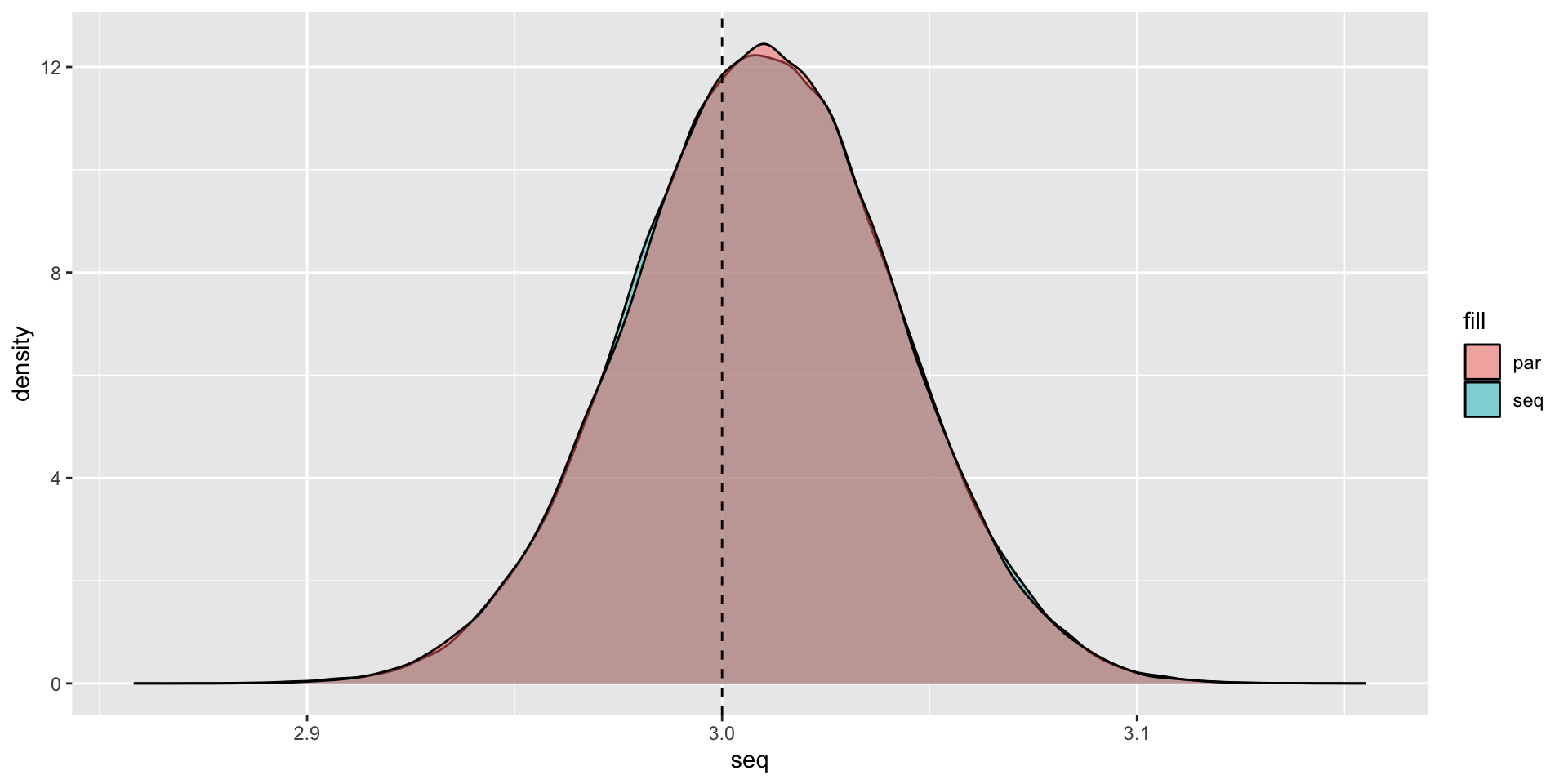
5.427 sec elapsed

After you run something in parallel, it’s good to set the plan back to sequential.

plan(sequential)

Plotting the Results

library(ggplot2)
tibble::tibble(true = 3, seq = slopes_seq, par = slopes_par) |>
  ggplot() +
  geom_density(aes(x = seq, fill = "seq"), alpha = 0.5) +
  geom_density(aes(x = par, fill = "par"), alpha = 0.5) +
  geom_vline(aes(xintercept = true), linetype = "dashed")

Plotting the Results

Packages that are already parallelized

A lot of speed performance from packages are from parallel processing.

library(data.table)

data.table 1.17.0 using 5 threads (see ?getDTthreads).  Latest news: r-datatable.com

This means that adding parallelization on top of data.table operations may not speed things up.

The fixest package also already parallelizes code for multiple fixed effect regressions.

So you have to be careful when paralleizing code that is already optimized.

Back to Functions

When Should You Use a Function?

Rule of Three

When you duplicate some code three times, you should write it as a function.

This is obviously a rule-of-thumb, but it’s a useful starting point.

You should also consider for your projects,

will I need to iterate over this step?
will I need to run robustness checks on this step?

Where Do You Write a Function?

A function has to be declared before you can use it.

So the simplest spot to put them is at the top of your R script.

## My functions
my_func <- function(x) {
  ## Does something
}
my_func2 <- function(x) {
  ## Does something else
}

## The rest of my code
data <- my_func(x)
my_func2(data)

But this can get overcrowded very quickly.

Sourcing Helper Scripts

A better solution is to store your functions in their own separate scripts.

Then you source() them into the main script, or wherever you need them.

helpers.R

## My functions
my_func <- function(x) {
  ## Does something
}

my_func2 <- function(x) {
  ## Does something else
}

main.R

source("helpers.R")

## The rest of my code
data <- my_func(x)
my_func2(data)

Creating an R Package

Another option is to create an R package for your functions.

This allows you to:

share your functions with others
reuse your functions across multiple projects
add documentation
add unit tests

You will create a simple test package as part of your homework assignment.

Live Coding Example

map(1:30, function(x){Sys.sleep(1)}, .progress = TRUE)

Live Coding Example - Parallelization on OSCAR

renv::install(c("tibble", "tictoc", "furrr"), prompt = FALSE)
library(tibble)
library(tictoc)
library(furrr)

availableCores()
n = 1e3 ## One thousand observations
set.seed(42)

data <- tibble::tibble(
  x = rnorm(n),
  y = 4 + 3 * x + rnorm(n)
)

bootstrap <- function(data, n_boot = 1e3) {
  boot_data <- data[sample(nrow(data), size = n_boot, replace = TRUE), ]
  m <- lm(y ~ x, data = boot_data)
  slope <- coef(m)[[2]]
  return(slope)
}

plan(multicore)

tic()
slopes_par <- future_map_dbl(1:1e5, ~ bootstrap(data), .options = furrr_options(seed = 42L))
toc()

plan(sequential)

tic()
slopes_par <- future_map_dbl(1:1e5, ~ bootstrap(data), .options = furrr_options(seed = 42L))
toc()

R Functions & Regressions

Functions

Functions

R is a Functional Language

Why use functions?

A Basic Function

Syntax

“Degenerate” functions

Variable Scope

Breaking Function Scope

Limiting Function Scope

Adding Additional Arguments

Setting a Default Argument

Ordering of Arguments

CRRA Utility

CRRA Utility

If-Else Statements within Functions

Printing out a function

Printing out a function

Anonymous Functions

Anonymous Functions

purrr::map() family

Map Family of Functions

Map Function

Using an Anonymous Function with map()

Using an Anonymous Function with map()

Multiline Anonymous Functions

map Return Types

Example with map_dbl()

Example with fredr package

Regression Functions

Regressions

Generating some example data

Estimating \(\beta\)

summary() for detailed information

Structure of lm() models

Summary also returns a list

Tidying model results

Subsets of data

Nesting tibbles

Running lm on nested tibbles

Tidying nested model results

Unnesting a tibble

Making a coefficient chart

Making a coefficient chart

Nesting Summary

Robust Standard Errors

Robust Standard Errors

Robust SE with estimatr

Changing the SE type

Panel Regressions

Panel Regressions

Panel data

Example Panel Data

Running OLS with fixest

Adding in fixed effects

Setting iid standard errors

Setting iid standard errors

Adding another variable

Running multiple fixed effects

Comparing models

Speed Comparison: fixest and Stata’s reghdfe

Parallel Processing

Parallel Processing

Parallel Processing

A Slow Function

Aside: Measuring Code Speed in R

Timing our Slow Function

Timing our Slow Function

Running in Parallel

Running in Parallel

furrr Package

Setting a Plan

Available Cores

Why Parallel Processing with map()?

Another Example: Bootstrapping

Bootstrap Function

Bootstrap in Parallel

Plotting the Results

Plotting the Results

`purrr::map()` family

Using an Anonymous Function with `map()`

Using an Anonymous Function with `map()`

`map` Return Types

Example with `map_dbl()`

Example with `fredr` package

`summary()` for detailed information

Structure of `lm()` models

Running `lm` on nested tibbles

Robust SE with `estimatr`

Running OLS with `fixest`

Speed Comparison: `fixest` and Stata’s `reghdfe`

`furrr` Package

Why Parallel Processing with `map()`?