R Data Wrangling: data.table
Using packages in R for data science
Matthew DeHaven
March 4, 2026
R environment details
R Library
R by default has one library of packages for all projects.
R Library
You can see where this library lives by calling,

Notice there are actually two library paths returned!
“User” Library
- For any packages you install
“System” Library
- For default packages when base R is installed
R Library
Installing packages puts them in User Library. Calling library() loads a package.
The Problems
There are two problems with R’s default package setup.
- All projects share the same library
- Updating a package for one project updates it for all
- It is not easy to record and recreate the exact packages used for a project
These are obviously related, which is why renv solves both.
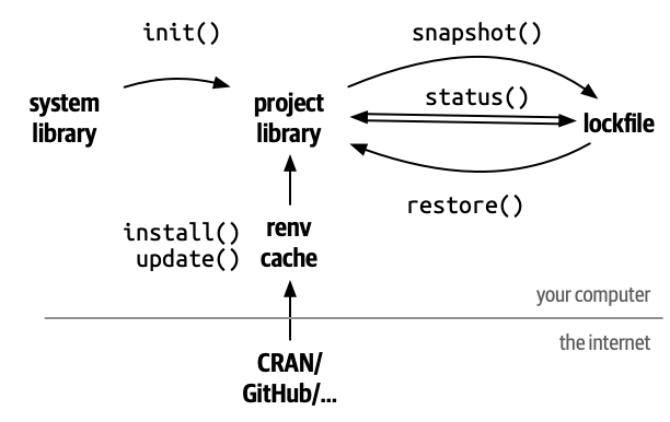
renv Separates Project Libraries
renv::init() makes isolated libraries for each project.
renv Cache
In order to avoid duplicate copies and downloads, renv stores a cache of all the packages it installs behind the scenes.
renv lockfile
The lockfile keeps tracks of what packages are used in a project.
It does not default to everything in the Project Library.
- You may have some packages you use just for development that are not needed for all of your code to run.
- An example of this is the
languageserverpackage
- An example of this is the
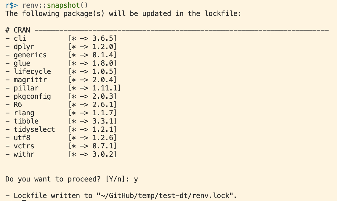
renv Record Packages to the Lockfile
In order to record a new package to the lockfile, run
This causes renv to search all of your project’s R files, see what packages are being used, and save the current version to the lockfile.
renv Status
To see if your lockfile is up-to-date, you can run
If everything is consistent, you will see this:

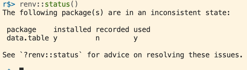
renv Status
To see if your lockfile is up-to-date, you can run
If everything a package is not tracked, but used, you will see:
renv Restore
If you open a project with a renv lockfile and want to recreate the package environment, run
You will see this in the next assignment.
renv Summary
data.table
data.table
Is another package focused on data science.
It’s goals:
- speed
- brevity
- no dependencies
In contrast to the tidyverse which is focused on readability.
Installing data.table
Again, we use renv to install data.table for any project we are using.
data.table objects
data.tables are a new object to replace data.frame.
Similar to tibbles, they have nicer default printing
               x           y
1    0.391037051  0.70672486
2   -0.797844018  1.27603101
3   -0.359482436  2.33528973
4   -0.237163332  0.19471902
5    0.690523500 -0.42378531
6    0.839320394  0.24693601
7    0.869473313  0.94007589
8    0.834238550 -1.45206334
9    0.704444826  0.31517017
10   1.857178038  0.34484943
11  -0.346629841 -0.20960703
12  -1.348117741 -0.43333636
13  -0.053063625  0.03998982
14  -0.837661905  1.70693872
15   0.235160981  0.29858022
16  -0.040019721  0.82758645
17   0.598917692  0.70845359
18   0.838430045  0.95846162
19  -0.217081609 -1.44102669
20   0.239927008  0.80564436
21  -0.683584208 -1.50964917
22  -0.452412301 -1.15454320
23  -0.546887431  0.03654041
24   1.143485195  0.58753254
25   0.655092187  1.25765603
26  -2.008748761 -0.71647941
27  -1.124809212 -1.46744876
28  -0.797140116  0.07858638
29  -0.902630700  1.19251838
30  -0.331246041  0.67247946
31  -0.498869023 -0.25941124
32  -1.291164502 -1.58580904
33  -0.185443174  1.71772606
34  -1.172406757  1.36257921
35   0.538753382 -0.32156718
36   1.754851154  1.04548331
37   0.571242475 -0.45254506
38   1.183745583  2.35805959
39  -0.071524635  0.72039114
40   2.213903828 -0.34642400
41   0.561433330  1.42152888
42   0.919708149  0.96938829
43   0.308319404 -1.73063926
44  -1.760492315  0.46158476
45  -1.310156433  0.77645704
46   0.769059596 -0.99961363
47   0.796739376 -0.53309785
48   0.018045191  0.71305882
49   0.939513320 -1.20582769
50  -0.764112200 -1.43367324
51  -1.262773849 -0.34772437
52   0.921321685  0.04391214
53  -1.294393423  0.74933623
54  -0.427052355 -0.13573626
55  -0.174637060 -1.42435498
56  -0.890281369  0.06967650
57  -1.214959957 -0.62391607
58  -0.623642438  1.81151848
59  -1.091010228  1.55703434
60  -0.917971935 -0.05189142
61  -1.321473628 -0.58969509
62  -1.873376647 -0.22787171
63  -0.659244271 -0.38643994
64  -0.116121593  1.27464443
65   0.178359454  0.86823984
66   0.622661575  0.32359083
67  -0.455876998 -0.51074616
68   1.232376107 -2.17389704
69   0.221093507 -1.57654844
70   0.317650421  2.99307244
71  -0.305121279  1.24824365
72   0.556446787  1.28195029
73   0.388784702 -0.58731265
74  -0.267789441 -0.32330193
75  -2.021060315 -2.42633102
76  -0.720577375  1.12797879
77  -0.807193919 -0.34797189
78   2.299893710 -1.69520745
79  -1.738654737 -0.78621392
80   0.078680302 -0.91597025
81   1.443552918 -0.12737549
82   0.215272448  0.71294022
83   1.690477443 -1.22851185
84   1.621934221  0.12748025
85  -0.138061040  1.71642865
86  -2.882525491 -0.50187316
87  -0.243444676  0.67322895
88  -2.195537979  1.90042596
89  -0.333587368  0.27050373
90   0.481517047 -0.99939382
91  -0.248646870  1.25953137
92  -0.067594891 -0.47346150
93   0.020474914  0.21328221
94   0.280744742  1.22446837
95   0.410260199  0.32041896
96   1.736610774 -0.67747606
97   0.949427209  1.85425533
98   1.054886829 -0.59644089
99  -0.485546005 -0.55949133
100 -0.066194377 -0.13316839
101  0.440781190 -2.31940301
102  1.771135378  1.42397182
103 -0.658486220 -0.53762804
104 -0.067216106 -0.37809847
105  0.868385292 -1.15369975
106 -0.167888490  1.13914743
107 -1.375105702  0.22484152
108 -0.805698093 -0.94410990
109  0.921195168 -0.60047808
110  0.638187056 -1.17519173
111 -1.322092027  0.61497970
112 -0.432022064  0.63432908
113  1.777501765  0.41680344
114  0.613973826 -0.88787392
115  0.393691140  0.32113845
116  0.761477884 -0.68333482
117 -0.503996768 -0.12435248
118 -0.381777068 -0.51950232
119 -3.570718958 -0.27007480
120  0.530932302 -1.63695068
121  0.938263515 -0.81525206
122  1.082399860 -0.40777629
123  0.840228605 -0.49733226
124 -0.660535840  0.45173782
125 -1.248263882 -0.36138639
126  1.730976261  0.13739870
127  0.483036157 -1.43151615
128  2.770251935 -0.81930598
129 -0.304846767 -0.44239061
130  0.989892767 -1.38892317
131 -1.282289285 -2.74581696
132 -0.071703881  0.89594907
133 -0.778305059  0.34888951
134 -0.711945238  0.22716615
135  0.477687178 -0.95322393
136  0.472164586  0.48337998
137  1.128484233 -0.23044453
138  1.463336419 -2.18832832
139 -1.726400828 -1.51130749
140  1.354573268  0.22307906
141 -1.563540941 -0.95865902
142  0.784883639 -0.26277337
143  0.447038299 -1.74509347
144  1.649248379  1.40564849
145 -0.024732417  0.31576528
146  0.374618014 -2.00527330
147  0.520441272  1.04045184
148  0.826118850 -0.11604969
149 -1.543415491  0.46384648
150 -0.357275864  1.23515919
151  0.579270150 -1.46637172
152  0.645195093  1.21648840
153 -0.957784807  0.31853750
154  0.017303839  0.72973881
155  0.881239459  0.90288465
156 -0.500219374 -0.19918925
157 -0.624313537  0.83157341
158  0.818231680  0.31046142
159  0.106953803  0.75397339
160 -0.576022561 -0.40330651
161  0.379822421 -2.10829582
162 -0.530939451  0.57972020
163  0.303890483 -0.31051805
164  0.313468805  1.04280470
165 -0.003517994 -0.22219718
166  0.630670561  2.36656695
167  0.314355195 -0.07397635
168  0.464017744  0.24959355
169  0.099589434  0.69112747
170 -1.554300553  0.96817679
171  1.350635667 -1.57128908
172  0.075102924 -0.02203584
173  0.202248756  0.58609342
174  0.986742644 -0.27794561
175 -1.243596077 -1.48023371
176  1.106496769  0.71884759
177 -0.757080542  1.10360372
178 -0.854065201  0.74137858
179 -0.745752376 -0.87978273
180  1.303124623  0.59804648
181  0.660346988  0.06912345
182  0.620740677 -0.19366783
183 -0.248433483  0.47915353
184 -0.425737118  0.78810226
185  0.380041465  0.20236721
186  0.278776077  0.33435084
187  0.570234569 -0.65076270
188  0.964952193 -0.23768627
189  1.581634958 -1.43782422
190  0.578149797  1.19945221
191  1.236180775 -0.55117243
192  0.563292243  0.53213623
193  0.901014214  0.49518964
194  0.816465456  0.74667707
195 -0.723993713 -1.12572641
196  1.153471919  1.79943287
197  0.163978362 -0.27611366
198  0.354244275 -0.02716657
199  0.383443888 -0.92011170
200 1.269924411 0.82574740 x y
<num> <num>
1: -0.84011814 -1.40068384
2: 0.03326073 -0.06354209
3: 1.27120495 -0.77549786
4: 0.48363083 -0.53904015
5: -0.09653324 -0.25541796
---
196: -2.37699653 -0.60439492
197: 0.78147175 -1.62531533
198: -0.34816658 1.14836532
199: 0.31235246 -0.36572910
200: 0.54380139 0.23651600data.table square brackets
Remember, from base R, than we can subset vectors, matrices, and data.frames using [i,j].
data.table square brackets
data.table takes square brackets a huge step further, by allowing
- filtering in the ‘i’ place
- new variable declaration in the ‘j’ place
We will look at each of these in turn.
data.table filtering
       a     b
   <num> <num>
1: -0.20   0.5
2:  0.10   0.0
3:  0.25  -0.2
4:  0.00   0.1
5: -0.30   0.3
What if we want all the values where “a” is less than 0?
data.table filtering
Instead we could do all the values where “a” is less than “b”.
data.table filtering
In fact, we can drop the comma, as data.table will assume that only one item is always the filtering argument.
tidyverse filtering equivalent
Here is a comparison of the data.table and tidyverse syntaxes side-by-side.
Pretty similar, but data.table is shorter.
data.table column subsetting
Remember: data.frame subsetting uses “i” for rows, and “j” for columns. data.table follows this.
For two columns, pass a list:
data.table variable declaration
What if we want to add a new column?
data.table does this using the column subsetting place, “j”.
:= is a data.table function representing “defined”.
Also called the “walrus” operator by some people.
data.table variable declaration
Would this work?
No.
data.table will assume we are using the “i” place for rows.
Error in `value[[3L]]()`:
! Operator := detected in i, the first argument inside DT[...], but is only valid in the second argument, j. Most often, this happens when forgetting the first comma (e.g. DT[newvar := 5] instead of DT[ , new_var := 5]). Please double-check the syntax. Run traceback(), and debugger() to get a line number.
data.table variable editing
We can use the exact same syntax to edit current columns.
data.table variable editing
Or to remove a column,
data.table conditional editing
What if we want to remove values of “b” that are less than 0?
We could conditionally declare values of “b” to be NA.
Summarizing with data.table
Remember in tidyverse we could write:
The equivalent in data.table is to pass a list .() to the “j” place:
Note that I had to make “mtcars” a data.table first.
Summarizing with data.table
Instead, I could simply make the mean a new column.
      mpg   cyl  disp    hp  drat    wt  qsec    vs    am  gear  carb      avg
    <num> <num> <num> <num> <num> <num> <num> <num> <num> <num> <num>    <num>
 1:  21.0     6 160.0   110  3.90 2.620 16.46     0     1     4     4 20.09062
 2:  21.0     6 160.0   110  3.90 2.875 17.02     0     1     4     4 20.09062
 3:  22.8     4 108.0    93  3.85 2.320 18.61     1     1     4     1 20.09062
 4:  21.4     6 258.0   110  3.08 3.215 19.44     1     0     3     1 20.09062
 5:  18.7     8 360.0   175  3.15 3.440 17.02     0     0     3     2 20.09062
 6:  18.1     6 225.0   105  2.76 3.460 20.22     1     0     3     1 20.09062
 7:  14.3     8 360.0   245  3.21 3.570 15.84     0     0     3     4 20.09062
 8:  24.4     4 146.7    62  3.69 3.190 20.00     1     0     4     2 20.09062
 9:  22.8     4 140.8    95  3.92 3.150 22.90     1     0     4     2 20.09062
10:  19.2     6 167.6   123  3.92 3.440 18.30     1     0     4     4 20.09062
11:  17.8     6 167.6   123  3.92 3.440 18.90     1     0     4     4 20.09062
12:  16.4     8 275.8   180  3.07 4.070 17.40     0     0     3     3 20.09062
13:  17.3     8 275.8   180  3.07 3.730 17.60     0     0     3     3 20.09062
14:  15.2     8 275.8   180  3.07 3.780 18.00     0     0     3     3 20.09062
15:  10.4     8 472.0   205  2.93 5.250 17.98     0     0     3     4 20.09062
16:  10.4     8 460.0   215  3.00 5.424 17.82     0     0     3     4 20.09062
17:  14.7     8 440.0   230  3.23 5.345 17.42     0     0     3     4 20.09062
18:  32.4     4  78.7    66  4.08 2.200 19.47     1     1     4     1 20.09062
19:  30.4     4  75.7    52  4.93 1.615 18.52     1     1     4     2 20.09062
20:  33.9     4  71.1    65  4.22 1.835 19.90     1     1     4     1 20.09062
21:  21.5     4 120.1    97  3.70 2.465 20.01     1     0     3     1 20.09062
22:  15.5     8 318.0   150  2.76 3.520 16.87     0     0     3     2 20.09062
23:  15.2     8 304.0   150  3.15 3.435 17.30     0     0     3     2 20.09062
24:  13.3     8 350.0   245  3.73 3.840 15.41     0     0     3     4 20.09062
25:  19.2     8 400.0   175  3.08 3.845 17.05     0     0     3     2 20.09062
26:  27.3     4  79.0    66  4.08 1.935 18.90     1     1     4     1 20.09062
27:  26.0     4 120.3    91  4.43 2.140 16.70     0     1     5     2 20.09062
28:  30.4     4  95.1   113  3.77 1.513 16.90     1     1     5     2 20.09062
29:  15.8     8 351.0   264  4.22 3.170 14.50     0     1     5     4 20.09062
30:  19.7     6 145.0   175  3.62 2.770 15.50     0     1     5     6 20.09062
31:  15.0     8 301.0   335  3.54 3.570 14.60     0     1     5     8 20.09062
32:  21.4     4 121.0   109  4.11 2.780 18.60     1     1     4     2 20.09062
      mpg   cyl  disp    hp  drat    wt  qsec    vs    am  gear  carb      avg
    <num> <num> <num> <num> <num> <num> <num> <num> <num> <num> <num>    <num>
data.table will spread any single value to the length of the table.
Multiple summaries
We can summarize multiple values or columns by simply adding arguments to .()
How do we do this by group?
We could use the filtering spot, “i”, and append each result
or…
Summarizing by group
We can use the “hidden” third square bracket argument: by=
     cyl      avg   med     n
   <num>    <num> <num> <int>
1:     6 19.74286  19.7     7
2:     4 26.66364  26.0    11
3:     8 15.10000  15.2    14
We can pass multiple columns to by using the short list: .()
data.table argument summary
dt[
i ,
j ,
by = ]
filtering rows
filtering columns, new columns, summarize
group by columns
tidyverse equivalent verbs
filter()
select(), mutate(), summarize()
groub_by()
Comparison
data.table syntax is more concise, but harder to read.
Class Activity
Class Activity
- Install and load
data.tablein a temporary workspace - Create a
data.tablewith columnsaandbof length 10 with random values - Add new column
cwhich is the sum ofaandb - Add a new column
dwhich is the product ofaandbwhenais greater than 0
Modify by Reference
Which should I use? data.table or tidyverse?
The main answer:
- personal preference (which syntax do you prefer?)
Second answer:
data.tableis much faster
- especially for large datasets
Speed comparison
A group that creates DuckDB (a fast database engine) does a regular speed comparison of different data manipulation tools across R, Python, Julia, and other languages:
Takeaway:
data.tableis much faster thandplyrfor data manipulation in R
Why is data.table faster?
- optimized for speed
- Modifies “by reference”
tidyverse functions instead “copy-on-modify”.
Modify by reference vs. copy
Copy-on-modify
- Creates a copy of the data
- Modifies the copy
- Returns the copy
Modify-in-place (modify “by reference”)
- References the data
- Modifies the original data
Avoids duplicating data, which is costly for your computer’s memory, especially with large datasets.
Modify by reference vs. copy
You may have noticed that I had to add an extra call to print data.tables after modifying them.
This is because the line dt[, y := c("a", "b")] doesn’t return anything.
Because it edited the data in place, not by creating a copy.
Dangers of editing by reference
Modifying by reference can be dangerous if you are not careful.
What happens to “dt” if we remove a column from “dt2”?
“dt” and “dt2” reference the same underlying data.
Dangers of editing by reference
If you truly want a new copy of a data.table, use
Converting to a data.table by reference
If you have a data.frame and want to convert it to a data.table, you can do this by reference as well.
Even Faster with Keys!
Keys
Keys provide some organization to your data.
This makes it much faster to later:
filter
group by
merge
data.table lets you add keys in a variety of ways.
You can also pass a vector of keys c("x", "y") to use.
What are keys?
Keys provide an index for the data.
Think of this like a phone book.
If you wanted to look my phone number up in the phone book,
you would search under “D” for DeHaven
you would not search the entire phone book!
When we tell data.table to use some columns as a key, it presorts and indexes the data on those columns.
Merging with data.table
For data.table all types of merges are handled by one function:
Key: <x>
        x     y     z
   <char> <int> <int>
1:      a     1     4
2:      c     3     5
By default, merge() does an “inner” join (matches in both datasets).
Merging with data.table
A “left” join,
Or an “outer” join
Non-matching column names
We can also be explicit about which columns to use from “x” and from “y”,
Key: <x>
        x     y     z
   <char> <int> <int>
1:      a     1     4
2:      c     3     5
But it’s probably better to clean up your column names before hand.
data.table pivots
A package tidyfast which offers
dt_pivot_longer()dt_pivot_wider()
to match the syntax of tidyr but with the speed of data.table.
data.table read / write functions
data.table has its own functions for reading and writing data, which are much faster than base R’s read.csv() and write.csv(), or tidyverse’s readr::read_csv() and readr::write_csv().
tidyverse or data.table?
tidyverse or data.table?
In practice, I (and many people) use a mix of both.
I personally prefer data.tables syntax for filtering, modifying columns, and summarizing.
If you really want the speed of data.table and the syntax of dplyr…
dtplyr
…there is a special package that combines the two!
dtplyr allows you to use all of the tidyverse verbs:
mutate()filter()groupby()
But behind the scenes runs everything using data.table.
A note on pipes
You can use pipes with data.table as well.
The underscore character _ is known as a “placeholder”,
and represents the object being piped.
Placeholder for pipes
The placeholder _ is normally used to assign the result of a pipe to a specific named argument in a function.
the append() function has two arguments: x and values.
Live Coding Example
Live Coding Example
Speed Comparison:
library(data.table)
library(dplyr)
library(tictoc)

nrows <- 1e7 # 10 million rows

dt <- data.table(
  id    = sample(letters, nrows, replace = TRUE),
  group = sample(1:100, nrows, replace = TRUE),
  value = rnorm(nrows)
)

tb <- tibble(
  id    = dt$id,
  group = dt$group,
  value = dt$value
)

tic("data.table")
dt[group == 1, value := 0]
toc()

tic("dplyr")
tb <- tb |> mutate(value = if_else(group == 1, 0, value))
toc()

dt2 <- copy(dt)
setkey(dt2, "group")

tic("data.table grouped")
dt2[group == 1, value := 0]
toc()