R Regressions
OLS, Fixed Effects, and IV
March 5, 2025
Lecture Goals
- How to run OLS in R
- Outputing nice tables of results
- Fixed effect models, panel regressions
tidymodels
Regressions
The workhorse of economics research is linear regression.
The simplest form of which is, \[ Y = \beta X + \epsilon \]
Given a set of values for \(Y\) and \(X\), we can estimate \(\hat{\beta}\).
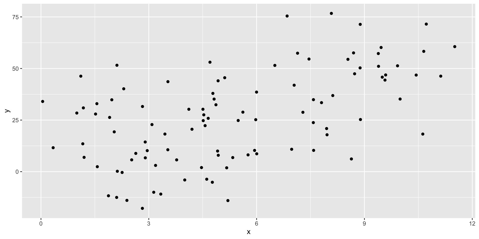
Generating some example data

Estimating \(\beta\)
R has a built in function for linear models: lm().
Call:
lm(formula = "y ~ x", data = tb)

Coefficients:
(Intercept)            x
      4.633        4.100
Printing the model returns only a few pieces of information, but there’s much more stored within.
summary() for detailed information
Call:
lm(formula = "y ~ x", data = tb)

Residuals:
    Min      1Q  Median      3Q     Max
-39.971 -14.708  -0.024  13.895  42.721

Coefficients:
            Estimate Std. Error t value Pr(>|t|)
(Intercept)    4.633      3.939   1.176    0.242
x              4.100      0.643   6.377 5.97e-09 ***
---
Signif. codes:  0 '***' 0.001 '**' 0.01 '*' 0.05 '.' 0.1 ' ' 1

Residual standard error: 18.85 on 98 degrees of freedom
Multiple R-squared:  0.2932,    Adjusted R-squared:  0.286
F-statistic: 40.66 on 1 and 98 DF,  p-value: 5.973e-09
Structure of lm() models
List of 12
 $ coefficients : Named num [1:2] 4.63 4.1
  ..- attr(*, "names")= chr [1:2] "(Intercept)" "x"
 $ residuals    : Named num [1:100] 26.09 -19.69 6.29 5.99 22.93 ...
  ..- attr(*, "names")= chr [1:100] "1" "2" "3" "4" ...
 $ effects      : Named num [1:100] -266.88 -120.21 1.64 7.22 24.75 ...
  ..- attr(*, "names")= chr [1:100] "(Intercept)" "x" "" "" ...
 $ rank         : int 2
 $ fitted.values: Named num [1:100] 14.1 26.5 13 45.3 48.6 ...
  ..- attr(*, "names")= chr [1:100] "1" "2" "3" "4" ...
 $ assign       : int [1:2] 0 1
 $ qr           :List of 5
  ..$ qr   : num [1:100, 1:2] -10 0.1 0.1 0.1 0.1 0.1 0.1 0.1 0.1 0.1 ...
  .. ..- attr(*, "dimnames")=List of 2
  .. .. ..$ : chr [1:100] "1" "2" "3" "4" ...
  .. .. ..$ : chr [1:2] "(Intercept)" "x"
  .. ..- attr(*, "assign")= int [1:2] 0 1
  ..$ qraux: num [1:2] 1.1 1.01
  ..$ pivot: int [1:2] 1 2
  ..$ tol  : num 1e-07
  ..$ rank : int 2
  ..- attr(*, "class")= chr "qr"
 $ df.residual  : int 98
 $ xlevels      : Named list()
 $ call         : language lm(formula = "y ~ x", data = tb)
 $ terms        :Classes 'terms', 'formula'  language y ~ x
  .. ..- attr(*, "variables")= language list(y, x)
  .. ..- attr(*, "factors")= int [1:2, 1] 0 1
  .. .. ..- attr(*, "dimnames")=List of 2
  .. .. .. ..$ : chr [1:2] "y" "x"
  .. .. .. ..$ : chr "x"
  .. ..- attr(*, "term.labels")= chr "x"
  .. ..- attr(*, "order")= int 1
  .. ..- attr(*, "intercept")= int 1
  .. ..- attr(*, "response")= int 1
  .. ..- attr(*, ".Environment")=<environment: 0x178a6ffa8>
  .. ..- attr(*, "predvars")= language list(y, x)
  .. ..- attr(*, "dataClasses")= Named chr [1:2] "numeric" "numeric"
  .. .. ..- attr(*, "names")= chr [1:2] "y" "x"
 $ model        :'data.frame':  100 obs. of  2 variables:
  ..$ y: num [1:100] 40.16 6.83 19.29 51.3 71.52 ...
  ..$ x: num [1:100] 2.3 5.34 2.04 9.92 10.72 ...
  ..- attr(*, "terms")=Classes 'terms', 'formula'  language y ~ x
  .. .. ..- attr(*, "variables")= language list(y, x)
  .. .. ..- attr(*, "factors")= int [1:2, 1] 0 1
  .. .. .. ..- attr(*, "dimnames")=List of 2
  .. .. .. .. ..$ : chr [1:2] "y" "x"
  .. .. .. .. ..$ : chr "x"
  .. .. ..- attr(*, "term.labels")= chr "x"
  .. .. ..- attr(*, "order")= int 1
  .. .. ..- attr(*, "intercept")= int 1
  .. .. ..- attr(*, "response")= int 1
  .. .. ..- attr(*, ".Environment")=<environment: 0x178a6ffa8>
  .. .. ..- attr(*, "predvars")= language list(y, x)
  .. .. ..- attr(*, "dataClasses")= Named chr [1:2] "numeric" "numeric"
  .. .. .. ..- attr(*, "names")= chr [1:2] "y" "x"
 - attr(*, "class")= chr "lm"
It’s just a big list!
You can access certain components (ex. m$residuals).
Summary also returns a list
List of 11
 $ call         : language lm(formula = "y ~ x", data = tb)
 $ terms        :Classes 'terms', 'formula'  language y ~ x
  .. ..- attr(*, "variables")= language list(y, x)
  .. ..- attr(*, "factors")= int [1:2, 1] 0 1
  .. .. ..- attr(*, "dimnames")=List of 2
  .. .. .. ..$ : chr [1:2] "y" "x"
  .. .. .. ..$ : chr "x"
  .. ..- attr(*, "term.labels")= chr "x"
  .. ..- attr(*, "order")= int 1
  .. ..- attr(*, "intercept")= int 1
  .. ..- attr(*, "response")= int 1
  .. ..- attr(*, ".Environment")=<environment: 0x178a6ffa8>
  .. ..- attr(*, "predvars")= language list(y, x)
  .. ..- attr(*, "dataClasses")= Named chr [1:2] "numeric" "numeric"
  .. .. ..- attr(*, "names")= chr [1:2] "y" "x"
 $ residuals    : Named num [1:100] 26.09 -19.69 6.29 5.99 22.93 ...
  ..- attr(*, "names")= chr [1:100] "1" "2" "3" "4" ...
 $ coefficients : num [1:2, 1:4] 4.633 4.1 3.939 0.643 1.176 ...
  ..- attr(*, "dimnames")=List of 2
  .. ..$ : chr [1:2] "(Intercept)" "x"
  .. ..$ : chr [1:4] "Estimate" "Std. Error" "t value" "Pr(>|t|)"
 $ aliased      : Named logi [1:2] FALSE FALSE
  ..- attr(*, "names")= chr [1:2] "(Intercept)" "x"
 $ sigma        : num 18.9
 $ df           : int [1:3] 2 98 2
 $ r.squared    : num 0.293
 $ adj.r.squared: num 0.286
 $ fstatistic   : Named num [1:3] 40.7 1 98
  ..- attr(*, "names")= chr [1:3] "value" "numdf" "dendf"
 $ cov.unscaled : num [1:2, 1:2] 0.04366 -0.00626 -0.00626 0.00116
  ..- attr(*, "dimnames")=List of 2
  .. ..$ : chr [1:2] "(Intercept)" "x"
  .. ..$ : chr [1:2] "(Intercept)" "x"
 - attr(*, "class")= chr "summary.lm"
It can be useful to access specific components with summary(m)$coefficients.
Tidying model results
broom is a package that tries to “tidy” model results into data.frames.
Let’s see what it does for our little model:
# A tibble: 2 × 5
  term        estimate std.error statistic       p.value
  <chr>          <dbl>     <dbl>     <dbl>         <dbl>
1 (Intercept)     4.63     3.94       1.18 0.242
2 x               4.10     0.643      6.38 0.00000000597
Much easier to work with!
The benefit of broom is that its written to create standardized results from many different models from many different packages.
Subsets of data
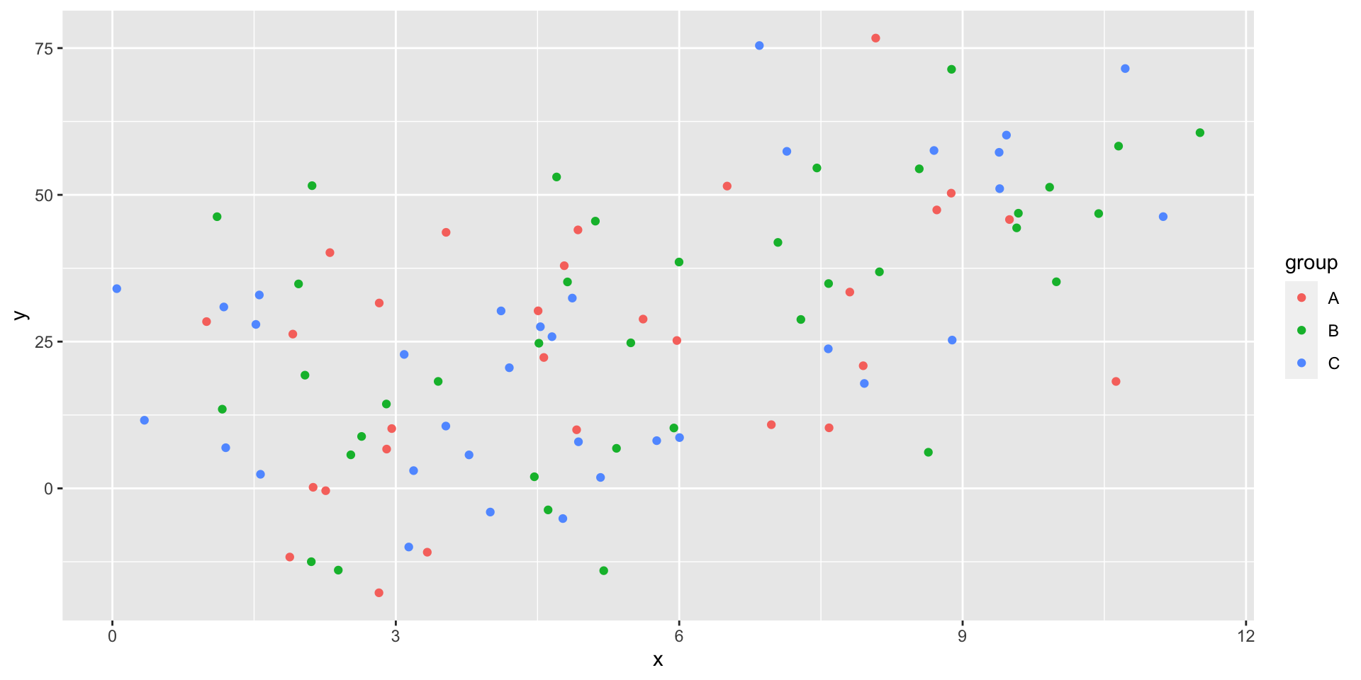
First, we are going to add some random groups to our data.

Nesting tibbles
What if we want to run multiple regressions, one on each group?
One option would be filter the data, then call lm three times.
Or we can set up nested tibbles.
We’ve separated our data into three tibbles, each stored as a row in our parent tibble.
Running lm on nested tibbles
Now we can use this nested format to run all three of our models at once.
# A tibble: 3 × 3
  group data              model
  <chr> <list>            <list>
1 A     <tibble [29 × 2]> <lm>
2 B     <tibble [37 × 2]> <lm>
3 C     <tibble [34 × 2]> <lm>
Now we have a column of lm models!
map is a function that takes a list or vector, applies a function to each element, and then returns a list or vector of the results.
In this case we are mapping the column “data”, to the function lm.
Tidying nested model results
Now we can tidy those models so we can contrast all of the results.
stb <- ntb |>
  mutate(model = map(data, function(tb) lm("y ~ x", data = tb) )) |>
  mutate(summary = map(model, broom::tidy))
stb
# A tibble: 3 × 4
group data model summary
<chr> <list> <list> <list>
1 A <tibble [29 × 2]> <lm> <tibble [2 × 5]>
2 B <tibble [37 × 2]> <lm> <tibble [2 × 5]>
3 C <tibble [34 × 2]> <lm> <tibble [2 × 5]>We have all of the model summaries now, but we need to unnest the tibble to easily compare them.
Unnesting a tibble
stb |>
  unnest(summary) |>
  select(-c("data", "model")) |>  ## dropping columns to fit on slide
  arrange(term)
# A tibble: 6 × 6
group term estimate std.error statistic p.value
<chr> <chr> <dbl> <dbl> <dbl> <dbl>
1 A (Intercept) 5.42 7.90 0.686 0.499
2 B (Intercept) 5.33 6.92 0.770 0.447
3 C (Intercept) 3.88 6.36 0.609 0.547
4 A x 3.74 1.38 2.72 0.0113
5 B x 4.10 1.05 3.89 0.000432
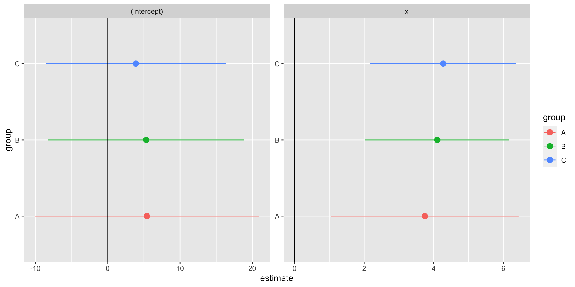
6 C x 4.27 1.07 4.00 0.000354We can now easily compare our three models’ \(\beta\) estimate for \(x\).
Making a coefficient chart
stb |>
  unnest(summary) |>
  ggplot() +
  geom_point(aes(
    x = estimate,
    y = group,
    color = group
  ),
    size = 3
  ) +
  geom_segment(aes(
    x = estimate - 1.96 * std.error,
    xend = estimate + 1.96 * std.error,
    y = group,
    yend = group,
    color = group
  )) +
  geom_vline(xintercept = 0) +
  facet_wrap(vars(term), scales = "free")
Making a coefficient chart

Nesting Summary
Pros
- A clean way to estimate multiple models
- Makes full use of
tidyversefunctions
- Easy to add more models, different subsets
Cons (or concerns)
- Duplicates data for each row
- This can be very costly for large datasets
Robust Standard Errors
Robust Standard Errors
As you know from econometrics class, you shold pretty much always use robust standard errors when you report results.
There are a couple of packages which support this in R,
Robust SE with estimatr
The package is written to match the syntax of lm().
Same point estimates, slightly different standard errors.
# A tibble: 2 × 5
  term        estimate std.error statistic       p.value
  <chr>          <dbl>     <dbl>     <dbl>         <dbl>
1 (Intercept)     4.63     3.94       1.18 0.242
2 x 4.10 0.643 6.38 0.00000000597 term estimate std.error statistic p.value conf.low conf.high df
1 (Intercept) 4.633091 4.0673715 1.139087 2.574435e-01 -3.438476 12.70466 98
2 x 4.100106 0.6251976 6.558096 2.574586e-09 2.859422 5.34079 98
outcome
1 y
2 yChanging the SE type
estimatr defaults to using “HC2” robust standard errors.
There are options for “HC0”, “HC1”, and “HC3”.
I can’t really tell you the importance of the small differences between these robust options. You can read more about the math for each here.
Matching STATA’s robust SE
If you want to match exactly the robust SEs reported in STATA, use “HC1” or “stata”
Panel Regressions
Panel Regressions
Fixed effects
Clustering
Panel data
Panel data has at least two dimensions
- time
- groups
- countries, states, people
This is in contrast to time series (just a time dimension) and cross-sectional data.
Example Panel Data
We are going to use the package gapminder to get our example panel data.
library(gapminder)
gapminder <- gapminder |> mutate(pop = pop / 1e6, gdpPercap = gdpPercap / 1e3)
gapminder
# A tibble: 1,704 × 6
country continent year lifeExp pop gdpPercap
<fct> <fct> <int> <dbl> <dbl> <dbl>
1 Afghanistan Asia 1952 28.8 8.43 0.779
2 Afghanistan Asia 1957 30.3 9.24 0.821
3 Afghanistan Asia 1962 32.0 10.3 0.853
4 Afghanistan Asia 1967 34.0 11.5 0.836
5 Afghanistan Asia 1972 36.1 13.1 0.740
6 Afghanistan Asia 1977 38.4 14.9 0.786
7 Afghanistan Asia 1982 39.9 12.9 0.978
8 Afghanistan Asia 1987 40.8 13.9 0.852
9 Afghanistan Asia 1992 41.7 16.3 0.649
10 Afghanistan Asia 1997 41.8 22.2 0.635
# ℹ 1,694 more rowsRunning OLS with fixest
Let’s predict life expectancy using GDP per capita.
OLS estimation, Dep. Var.: lifeExp
Observations: 1,704
Standard-errors: IID
             Estimate Std. Error  t value  Pr(>|t|)
(Intercept) 53.955561   0.314995 171.2902 < 2.2e-16 ***
gdpPercap    0.764883   0.025790  29.6577 < 2.2e-16 ***
---
Signif. codes:  0 '***' 0.001 '**' 0.01 '*' 0.05 '.' 0.1 ' ' 1
RMSE: 10.5   Adj. R2: 0.340326
We could easily have estimated this with
lm()orlm_robust()
Adding in fixed effects
Let’s add fixed effects for each continent.
OLS estimation, Dep. Var.: lifeExp
Observations: 1,704
Fixed-effects: continent: 5
Standard-errors: Clustered (continent)
          Estimate Std. Error t value Pr(>|t|)
gdpPercap  0.44527   0.101302 4.39546 0.011733 *
---
Signif. codes:  0 '***' 0.001 '**' 0.01 '*' 0.05 '.' 0.1 ' ' 1
RMSE: 8.37531     Adj. R2: 0.578106
                Within R2: 0.174557
Super easy to run!
Notice that it automatically clustered our standard errors to “continent” as well. What if we don’t want that? When Should You Adjust Standard Errors for Clustering (Abadie, Athey, Imbens, Woolridge 2017)
Setting iid standard errors
We can be explicit about standard errors using the “vcov=” argument.
OLS estimation, Dep. Var.: lifeExp
Observations: 1,704
Fixed-effects: continent: 5
Standard-errors: IID
          Estimate Std. Error t value  Pr(>|t|)
gdpPercap  0.44527   0.023498 18.9493 < 2.2e-16 ***
---
Signif. codes:  0 '***' 0.001 '**' 0.01 '*' 0.05 '.' 0.1 ' ' 1
RMSE: 8.37531     Adj. R2: 0.578106
                Within R2: 0.174557
Setting iid standard errors
We can also have clustered standard errors without including fixed effects.
OLS estimation, Dep. Var.: lifeExp
Observations: 1,704
Standard-errors: Clustered (continent)
             Estimate Std. Error  t value   Pr(>|t|)
(Intercept) 53.955561   4.586864 11.76306 0.00029883 ***
gdpPercap    0.764883   0.290197  2.63574 0.05783770 .
---
Signif. codes:  0 '***' 0.001 '**' 0.01 '*' 0.05 '.' 0.1 ' ' 1
RMSE: 10.5   Adj. R2: 0.340326
Adding another variable
I want to add another fixed effect, so I’m going to add a new column for countries with big vs. small populations.
Running multiple fixed effects
We can add multiple fixed effects with the same syntax as adding more regressors.
OLS estimation, Dep. Var.: lifeExp
Observations: 1,704
Fixed-effects: continent: 5,  big_small: 2
Standard-errors: Clustered (continent)
          Estimate Std. Error t value  Pr(>|t|)
gdpPercap 0.453664   0.094069 4.82266 0.0085066 **
---
Signif. codes:  0 '***' 0.001 '**' 0.01 '*' 0.05 '.' 0.1 ' ' 1
RMSE: 8.32322     Adj. R2: 0.583092
                Within R2: 0.180956
Comparing models
fixest has a very nice function to print multiple models:
                              mf              mfiid             mf2fe
Dependent Var.:          lifeExp            lifeExp           lifeExp

gdpPercap       0.4453* (0.1013) 0.4453*** (0.0235) 0.4537** (0.0941)
Fixed-Effects:  ---------------- ------------------ -----------------
continent                    Yes                Yes               Yes
big_small                     No                 No               Yes
_______________ ________________ __________________ _________________
S.E. type          by: continent                IID     by: continent
Observations               1,704              1,704             1,704
R2                       0.57934            0.57934           0.58456
Within R2                0.17456            0.17456           0.18096
---
Signif. codes: 0 '***' 0.001 '**' 0.01 '*' 0.05 '.' 0.1 ' ' 1
Instrumental Variables
Instrumental Variables
If you are lucky enough to have an instrument you will want to use it!
We’ll look at how to estimate IV with the fixest package.
But you can also use,
estimatr::iv_robust()ivreg::ivreg()
fixest syntax
fixest uses a specific syntax for the formula argument:
y ~ ex | fe | en ~ in
ydependent variableexexogenous independent variablesfefixed effect variablesenendogenous independent variables- i.e. things that need an instrument
ininstrumental variables
fixest syntax options
We have already seen you can use,
y ~ ex | fe
You can also just use the instrument slot,
y ~ ex | en ~ in
Let’s try an example.
Example IV with fixest
Let’s add “population” as an independent variable and instrument it with the “big_small” variable we constructed. 1
TSLS estimation, Dep. Var.: lifeExp, Endo.: pop, Instr.: big_small
Second stage: Dep. Var.: lifeExp
Observations: 1,704
Standard-errors: IID
             Estimate Std. Error   t value  Pr(>|t|)
(Intercept) 51.643119   0.515593 100.16255 < 2.2e-16 ***
fit_pop      0.073201   0.011262   6.49992 1.053e-10 ***
gdpPercap    0.785063   0.030712  25.56198 < 2.2e-16 ***
---
Signif. codes:  0 '***' 0.001 '**' 0.01 '*' 0.05 '.' 0.1 ' ' 1
RMSE: 12.4   Adj. R2: 0.074081
F-test (1st stage), pop: stat = 115.4, p < 2.2e-16  , on 1 and 1,701 DoF.
Wu-Hausman: stat = 49.4, p = 2.988e-12, on 1 and 1,700 DoF.Fixed Effects, Clustering, and IV
And an example of everything at once.
TSLS estimation, Dep. Var.: lifeExp, Endo.: pop, Instr.: big_small
Second stage: Dep. Var.: lifeExp
Observations: 1,704
Fixed-effects: continent: 5
Standard-errors: Clustered (continent)
          Estimate Std. Error t value Pr(>|t|)
fit_pop   0.041589   0.029410 1.41410 0.230229
gdpPercap 0.472082   0.082549 5.71882 0.004626 **
---
Signif. codes:  0 '***' 0.001 '**' 0.01 '*' 0.05 '.' 0.1 ' ' 1
RMSE: 9.0883     Adj. R2: 0.502924
               Within R2: 0.028035
F-test (1st stage), pop: stat = 85.4, p < 2.2e-16 , on 1 and 1,701 DoF.
             Wu-Hausman: stat = 15.9, p = 6.927e-5, on 1 and 1,696 DoF.
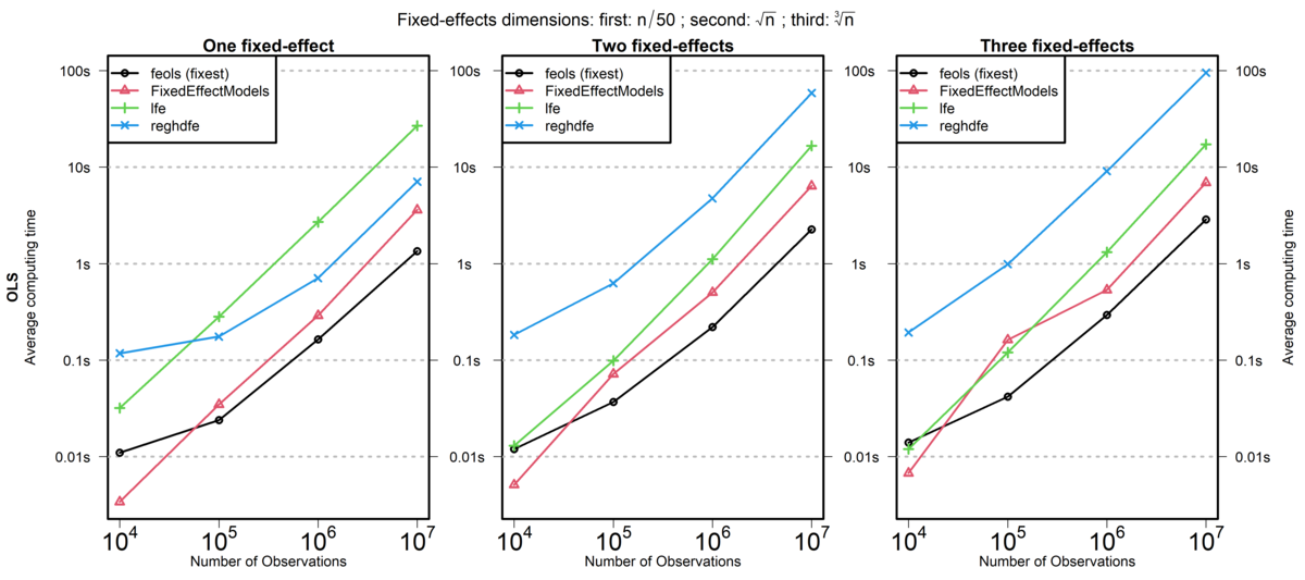
Speed Comparison: fixest and Stata’s reghdfe

lfe is another R package, reghdfe is a Stata package, and FixedEffectModels is a Julia package.
Source: fixest documentation (comparison run in 2020)
Tables
Making Tables in R
There are many options for making regression tables
modelsummarystargazergtsummaryfixest::etablefor fixest models
We will take a look at the modelsummary package.
Installing and loading
First we need to install and load the package.
And then we need to load it.
modelsummary Data Summaries
We can easily get some summary information about any dataset with:
modelsummary Data Summaries
| Unique | Missing Pct. | Mean | SD | Min | Median | Max | Histogram | |
|---|---|---|---|---|---|---|---|---|
| mpg | 25 | 0 | 20.1 | 6.0 | 10.4 | 19.2 | 33.9 |  |
| cyl | 3 | 0 | 6.2 | 1.8 | 4.0 | 6.0 | 8.0 |  |
| disp | 27 | 0 | 230.7 | 123.9 | 71.1 | 196.3 | 472.0 |  |
| hp | 22 | 0 | 146.7 | 68.6 | 52.0 | 123.0 | 335.0 |  |
| drat | 22 | 0 | 3.6 | 0.5 | 2.8 | 3.7 | 4.9 |  |
| wt | 29 | 0 | 3.2 | 1.0 | 1.5 | 3.3 | 5.4 |  |
| gear | 3 | 0 | 3.7 | 0.7 | 3.0 | 4.0 | 5.0 |  |
| vs | 2 | 0 | 0.4 | 0.5 | 0.0 | 0.0 | 1.0 |  |
modelsummary Model Summaries
To make regression tables we use
modelsummary Model Summaries
And we can combine multiple models by passing them as a list.
modelsummary Model Summaries
You can name them as well.
modelsummary(list(`Fixed Effects` = mf, `No Cluster` = mfiid, `Two FE` = mf2fe, `IV` = mall), gof_map = c("nobs", "r.squared"))| Fixed Effects | No Cluster | Two FE | IV | |
|---|---|---|---|---|
| gdpPercap | 0.445 | 0.445 | 0.454 | 0.472 |
| (0.101) | (0.023) | (0.094) | (0.083) | |
| fit_pop | 0.042 | |||
| (0.029) | ||||
| Num.Obs. | 1704 | 1704 | 1704 | 1704 |
| R2 | 0.579 | 0.579 | 0.585 | 0.505 |
modelsummary All Goodness of Fit
modelsummary Output to LaTeX
\begin{table}
\centering
\begin{tblr}[         %% tabularray outer open
]                     %% tabularray outer close
{                     %% tabularray inner open
colspec={Q[]Q[]},
column{1}={halign=l,},
column{2}={halign=c,},
hline{6}={1,2}{solid, 0.05em, black},
}                     %% tabularray inner close
\toprule
& (1) \\ \midrule %% TinyTableHeader
(Intercept) & \num{4.633}    \\
& (\num{3.939})  \\
x           & \num{4.100}    \\
& (\num{0.643})  \\
Num.Obs.    & \num{100}      \\
R2          & \num{0.293}    \\
R2 Adj.     & \num{0.286}    \\
AIC         & \num{875.1}    \\
BIC         & \num{882.9}    \\
Log.Lik.    & \num{-434.547} \\
RMSE        & \num{18.66}    \\
\bottomrule
\end{tblr}
\end{table}
modelsummary Output to LaTeX
You should never be manually writing your LaTeX tables.
- You may make a mistake
- They will get out of sync
Instead, use a package like modelsummary and automate
Fully Custom Tables
Sometimes you will want to construct a unique table and have full control over the layout.
Again, there are many possible packages to use:
kableExtragtflextableDT
We will take a look at the package gt.
Installing and loading
First we need to install the package.
And then load it.
Summarizing Some Data
gp_summ <-
  gapminder |>
  filter(year == max(year)) |>
  group_by(continent) |>
  summarize(pop = sum(pop), gdpPercap = mean(gdpPercap), lifeExp = mean(lifeExp))
gp_summ
# A tibble: 5 × 4
continent pop gdpPercap lifeExp
<fct> <dbl> <dbl> <dbl>
1 Africa 930. 3.09 54.8
2 Americas 899. 11.0 73.6
3 Asia 3812. 12.5 70.7
4 Europe 586. 25.1 77.6
5 Oceania 24.5 29.8 80.7A Simple Table
gt will print all of the cells in your data.frame.
Adding Row Groups
gt(gp_summ) |>
  tab_row_group(
    label = "Western Hemisphere",
    rows = 2
  ) |>
  tab_row_group(
    label = "Eastern Hemisphere",
    rows = c(1, 3:5)
)| continent | pop | gdpPercap | lifeExp |
|---|---|---|---|
| Eastern Hemisphere | |||
| Africa | 929.53969 | 3.089033 | 54.80604 |
| Asia | 3811.95383 | 12.473027 | 70.72848 |
| Europe | 586.09853 | 25.054482 | 77.64860 |
| Oceania | 24.54995 | 29.810188 | 80.71950 |
| Western Hemisphere | |||
| Americas | 898.87118 | 11.003032 | 73.60812 |
Adding Column Groups
| continent | Economic Variables | ||
|---|---|---|---|
| pop | gdpPercap | lifeExp | |
| Africa | 929.53969 | 3.089033 | 54.80604 |
| Americas | 898.87118 | 11.003032 | 73.60812 |
| Asia | 3811.95383 | 12.473027 | 70.72848 |
| Europe | 586.09853 | 25.054482 | 77.64860 |
| Oceania | 24.54995 | 29.810188 | 80.71950 |
Convert gt to LaTeX
\begin{longtable}{crrr}
\toprule
continent & pop & gdpPercap & lifeExp \\
\midrule\addlinespace[2.5pt]
Africa & 929.53969 & 3.089033 & 54.80604 \\
Americas & 898.87118 & 11.003032 & 73.60812 \\
Asia & 3811.95383 & 12.473027 & 70.72848 \\
Europe & 586.09853 & 25.054482 & 77.64860 \\
Oceania & 24.54995 & 29.810188 & 80.71950 \\
\bottomrule
\end{longtable}
Save a gt to a file
Perhaps even better is saving the table to a “.tex” file.
gt Summary
From gt’s documentation.
Summary
Lecture Summary
- Fitting basic OLS models:
lm() - Robust Standard Errors:
estimatr::lm_robust() - Tidying model output:
broom::tidy() - Fixed Effects:
fixest::feols- and Clustered Standard Errors
- and Instrument Variables
- Tables
modelsummarygt- Outputting to LaTeX
Live Coding Example
- Estimate a linear model with the
irisdataset - Show the
predictfunction
Coding Exercise
- Open a practice R session
- Load the
mtcarsdataset - Estimate a linear model of
mpgonwtwith robust standard errors - Use
broomto tidy the results