[1] 8R Functions
A functional approach to programming
Matthew DeHaven
March 10, 2025
Lecture Summary
What is a function?
- Syntax
- Variable scope
Anonymous functions
purrr::map()familyParallel processing
Functions
Functions
Functions…
- take input(s)
- do something
- return an ouput
R is a Functional Language
R, at its heart, is a functional programming (FP) language. This means that it provides many tools for the creation and manipulation of functions. In particular, R has what’s known as first class functions. You can do anything with functions that you can do with vectors: you can assign them to variables, store them in lists, pass them as arguments to other functions, create them inside functions, and even return them as the result of a function. Hadley Wickham, Advanced R
Why use functions?
Functions make your code
- more flexible
- less repetitive
- more readable (potentially)
A Basic Function
Here is a basic, if not exciting, function:
- Take inputs
- Do something
- Return output
Syntax
Functions are always declared using the function function(),
followed by curly braces { } which demark what the function actually does.
Most functions will end with a return() call, though this is not strictly required.
“Degenerate” functions
Which is just to show that technically inputs and outputs are not necessary.
In fact, we could make a function that does nothing…not very useful.
Variable Scope
Functions have their own “environment” for variables.
[1] "Outside function"Even if we call our function, the value for cubed is not overwritten in our R session environment.
Breaking Function Scope
<<- breaks the scope of a function and affects vaiables outside
[1] 27[1] 27But this is a really bad idea.
You should only allow functions to affect your session by returning values.
Otherwise, it is very confusing to tell what is changing a variable.
Limiting Function Scope
Technically, you can use a variable defined outside a function inside a function.
But this is also a bad idea.
Functions are meant to be flexible and portable
By relying on a session variable we’ve made this function dependent on the current setting.
Adding Additional Arguments
Instead, we should pass beta as an additional argument for our function.
Setting a Default Argument
When declaring a function, you can set a default value for an argument.
That default value will be used unless you specify a new value to overwrite it.
Ordering of Arguments
Functions assume unlabelled arguments are given in the order they were declared.
i.e. the first argument is our consumption value, and the second is our beta.
You can always be explicit about function arguments as well.
CRRA Utility
Let’s declare a CRRA utility function,
\[ U(C) = \beta \frac{C^{1-\gamma}}{1-\gamma} \]
In our code, this looks like
CRRA Utility
Let’s declare a CRRA utility function,
\[ U(C) = \beta \frac{C^{1-\gamma}}{1-\gamma} \]
What happens if we run when gamma = 1?
If you paid attention in Macro, then you know that CRRA utility with \(\gamma \rightarrow 1\) converges to log utility.
If-Else Statements within Functions
We can implement this with an if-else statement within our function.
Now our function works in both cases:
Printing out a function
We can always inspect the actual code for a function by calling it without the parentheses ().
Printing out a function
This works for functions from other packages too.
function(x, n = 1L, default = NULL, order_by = NULL, ...) {
  if (inherits(x, "ts")) {
    abort("`x` must be a vector, not a <ts>, do you want `stats::lag()`?")
  }
  check_dots_empty0(...)

  check_number_whole(n)
  if (n < 0L) {
    abort("`n` must be positive.")
  }

  shift(x, n = n, default = default, order_by = order_by)
}
<bytecode: 0x125255220>
<environment: namespace:dplyr>
Anonymous Functions
Anonymous functions are functions that do not have a name.

Anonymous Functions
Anonymous functions are functions that do not have a name.
This means they are not stored as a variable that you can use over again, but exist only for a moment.
For functions that only take one line, you can drop the curly brackets.
When would we use this?
purrr::map() family
Map Family of Functions
We saw briefly the *apply() family of base R functions (when we were looking at loops).
The map() family is the tidyverse equivalent and are nicer to use.
Map Function
The map() function always
- takes a vector (or list) for input
- calls a function on each element
- returns a list as the result
Using an Anonymous Function with map()
This is an example where we may want to declare an anonymous function.
Using an Anonymous Function with map()
And again, because our function is only one line, we could drop the curly braces.
Multiline Anonymous Functions
Conversely, you could have a multiline anonymous function.
[[1]]
      mpg             cyl             disp
 Min.   :10.40   Min.   :4.000   Min.   : 71.1
 1st Qu.:15.43   1st Qu.:4.000   1st Qu.:120.8
 Median :19.20   Median :6.000   Median :196.3
 Mean   :20.09   Mean   :6.188   Mean   :230.7
 3rd Qu.:22.80   3rd Qu.:8.000   3rd Qu.:326.0
 Max.   :33.90   Max.   :8.000   Max.   :472.0

[[2]]
  Sepal.Length    Sepal.Width     Petal.Length
 Min.   :4.300   Min.   :2.000   Min.   :1.000
 1st Qu.:5.100   1st Qu.:2.800   1st Qu.:1.600
 Median :5.800   Median :3.000   Median :4.350
 Mean   :5.843   Mean   :3.057   Mean   :3.758
 3rd Qu.:6.400   3rd Qu.:3.300   3rd Qu.:5.100
 Max.   :7.900   Max.   :4.400   Max.   :6.900
map Return Types
By default, map() will always return a list.
It does not know the datatype of the objects you are returning,
- and a list works with any data type and with a mix of data types.
If you do know your datatype, you could use…
map_lgl()map_int()map_dbl()map_chr()
- Which will all return a vector of that data type.
Example with map_dbl()
Using our prior map example,
map_dfr() for data.frames
We saw before that the map_dfr() was convenient for working with fredr package.
# A tibble: 2,090 × 5
   date       series_id value realtime_start realtime_end
   <date>     <chr>     <dbl> <date>         <date>
 1 1948-01-01 UNRATE      3.4 2025-03-07     2025-03-07
 2 1948-02-01 UNRATE      3.8 2025-03-07     2025-03-07
 3 1948-03-01 UNRATE      4   2025-03-07     2025-03-07
 4 1948-04-01 UNRATE      3.9 2025-03-07     2025-03-07
 5 1948-05-01 UNRATE      3.5 2025-03-07     2025-03-07
 6 1948-06-01 UNRATE      3.6 2025-03-07     2025-03-07
 7 1948-07-01 UNRATE      3.6 2025-03-07     2025-03-07
 8 1948-08-01 UNRATE      3.9 2025-03-07     2025-03-07
 9 1948-09-01 UNRATE      3.8 2025-03-07     2025-03-07
10 1948-10-01 UNRATE      3.7 2025-03-07     2025-03-07
# ℹ 2,080 more rows
map_dfr() for data.frames
We saw before that the map_dfr() was convenient for working with fredr package.
This map function returns data.frames (tibbles) and then combines them by rbind-ing them.
rbind()takes two data.frames and stacks them on top of each othercbind()takes two data.frames and stacks them beside one another
purrr Suggests a Different Function
purrr notes in their documentation that map_dfr() has been superseded. Instead, we should use…
# A tibble: 2,090 × 5
   date       series_id value realtime_start realtime_end
   <date>     <chr>     <dbl> <date>         <date>
 1 1948-01-01 UNRATE      3.4 2025-03-07     2025-03-07
 2 1948-02-01 UNRATE      3.8 2025-03-07     2025-03-07
 3 1948-03-01 UNRATE      4   2025-03-07     2025-03-07
 4 1948-04-01 UNRATE      3.9 2025-03-07     2025-03-07
 5 1948-05-01 UNRATE      3.5 2025-03-07     2025-03-07
 6 1948-06-01 UNRATE      3.6 2025-03-07     2025-03-07
 7 1948-07-01 UNRATE      3.6 2025-03-07     2025-03-07
 8 1948-08-01 UNRATE      3.9 2025-03-07     2025-03-07
 9 1948-09-01 UNRATE      3.8 2025-03-07     2025-03-07
10 1948-10-01 UNRATE      3.7 2025-03-07     2025-03-07
# ℹ 2,080 more rows
Which has the same result.
Parallel Processing
Parallel Processing
Sequential processing (default) is when code is run on one “core”.
Parallel Processing
Parallel processing splits operations over multiple “cores”.
A Slow Function
Imagine we had some slow code that we wanted to run multiple times.
Aside: Measuring Code Speed in R
We will use the package tictoc to measure the time it takes to run our function.
If you want more systematic code profiling, you can use the profvis or microbenchmark packages.
Timing our Slow Function
Now we can see how long our slow function takes to run.
Timing our Slow Function
And if we ran it multiple times…
Running in Parallel
If we have a multi-core machine, we can run this slow code in parallel!
Running in Parallel
And this can scale up!
furrr Package
The package we used is called furrr for future and purrr.
future is a package that allows you to run code in parallel.
Documentation:
Setting a Plan
The plan() function sets the parallel processing plan.
sequentialruns code sequentially (the default)multisessionruns code in parallel using multiple R sessionsmulticoreruns code in parallel using multiple cores- Only works on Unix-based systems (Linux, MacOS) and not in Rstudio
Available Cores
You can check how many cores you have available on your machine.
Why Parallel Processing with map()?
Remember that map() is a function that applies another function to each element of a list or vector.
This is always a parallel-izable task.
This is one reason it is good to use map() over a for loop.
- easier to parallelize in the future
Another Example: Bootstrapping
Bootstrapping is a common econometric task that can be easily parallelized.
Let’s generate some data.
Bootstrap Function
To get some standard errors, let’s bootstrap the data.
Bootstrap in Parallel
Or we can run it in parallel!
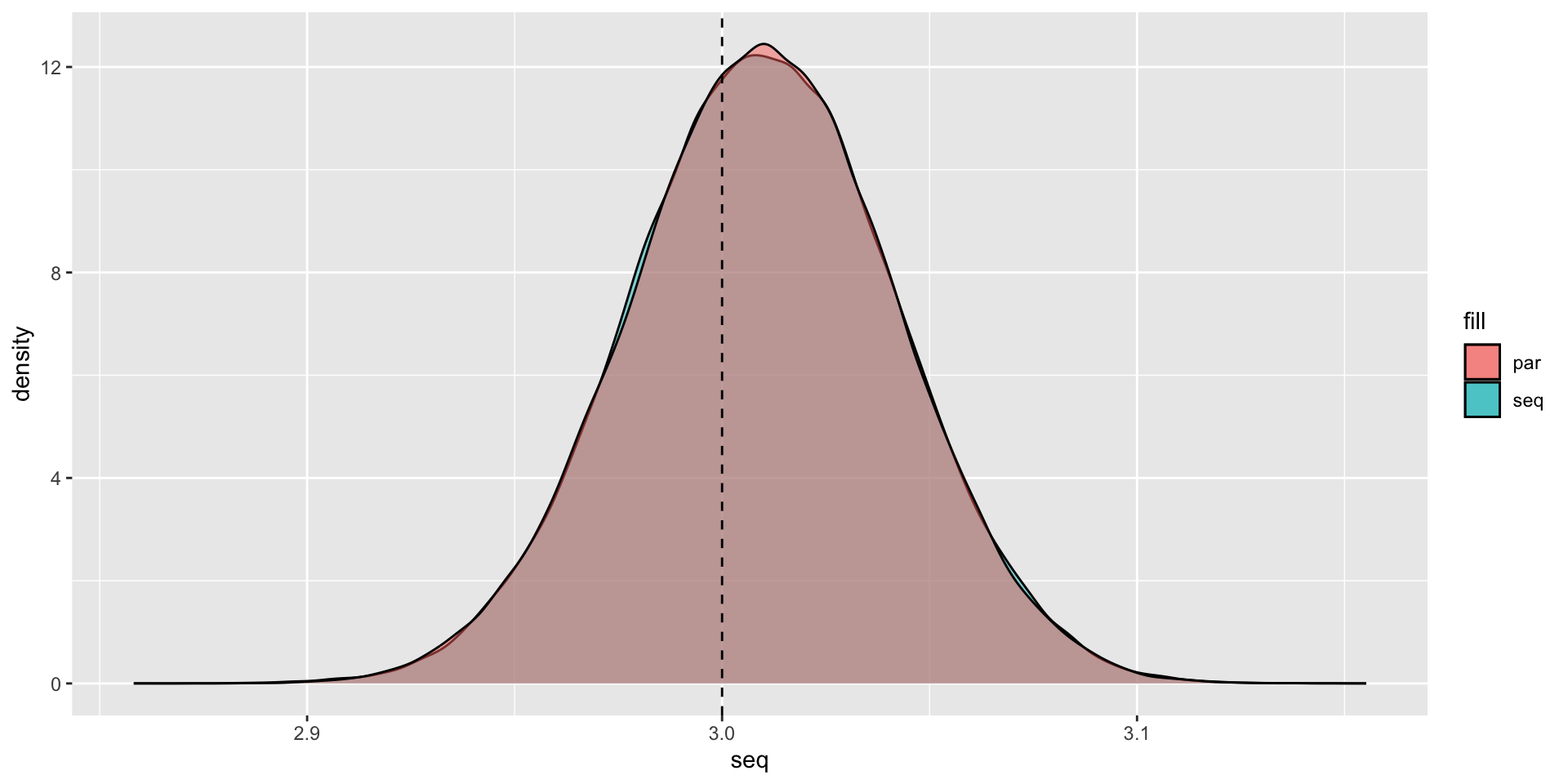
Plotting the Results
Plotting the Results
Packages that are already parallelized
A lot of the speed perforamance you see from packages are from parallel processing.
data.table 1.17.0 using 5 threads (see ?getDTthreads). Latest news: r-datatable.comThis means that adding parallelization on top of data.table operations may not speed things up.
The fixest package also already parallelizes code for multiple fixed effect regressions.
So you have to be careful when paralleizing code that is already optimized.
Back to Functions
When Should You Use a Function?
Rule of Three
- When you duplicate some code three times, you should write it as a function.
This is obviously a rule-of-thumb, but it’s a useful starting point.
You should also consider for your projects,
- will I need to iterate over this step?
- will I need to run robustness checks on this step?
Where Do You Write a Function?
A function has to be declared before you can use it.
So the simplest spot to put them is at the top of your R script.
But this can get overcrowded very quickly.
Sourcing Helper Scripts
A better solution is to store your functions in their own separate scripts.
Then you source() them into the main script, or wherever you need them.
Or, you could put your functions into their own package…
- this will be a whole lecture topic!
Lecture Summary
Lecture Summary
- Functions
- Anonymous functions
purrr::map()familysource()
- Parallel Processing
furrrpackage
Live Coding Example
- Writing a basic utility function
- Using
map()to apply it to a vector - Setting a progress bar with
.progressargument
Coding Exercise
- Write a slow function (using
Sys.sleep()) - Use
map()to apply it to a vector - Use
future_map()to apply it in parallel