R Data Wrangling: data.table
Using packages in R for data science
Matthew DeHaven
February 12, 2025
Lecture Summary
- Talking more about
renv data.table
More renv
R Library
R by default has one library of packages for all projects.
R Library
You can see where this library lives by calling,

Notice there are actually two library paths returned!
“User” Library
- For any packages you install
“System” Library
- For default packages when base R is installed
R Library
Installing packages puts them into the User Library. Calling library() loads a package.
The Problems
There are two problems with R’s default package setup.
- All projects share the same library
- Updating a package for one project updates it for all
- It is not easy to record and recreate the exact packages used for a project
These are obviously related, which is why renv solves both.
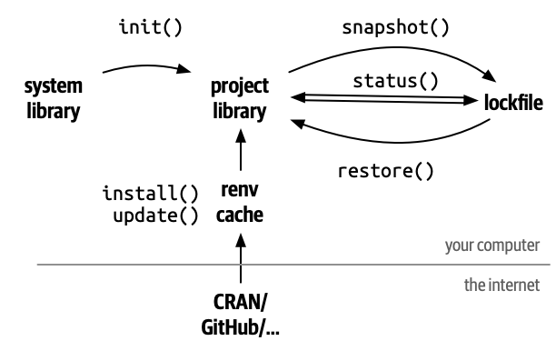
renv Separates Project Libraries
renv::init() makes isolated libraries for each project.
renv Cache
In order to avoid duplicate copies and downloads, renv stores a cache of all the packages it installs behind the scenes.
This solves projects changing each other’s packages, but does not yet give us any way to track and restore packages.
renv lockfile
The lockfile keeps tracks of what packages are used in a project.
It does not default to everything in the Project Library.
- You may have some packages you use just for development that are not needed for all of your code to run.
- An example of this is the
languageserverpackage
renv Record Packages to the Lockfile
In order to record a new package to the lockfile, run
This causes renv to search all of your project’s R files, see what packages are being used, and save the current version to the lockfile.
renv Status
To see if your lockfile is up-to-date, you can run
renv will also tell you if everything is up-to-date when you launch a new R terminal.
renv Restore
If you open a project with a renv lockfile and want to recreate the package environment, run
You will see this in the next assignment.
renv Summary
data.table
data.table
Is another package focused on data science.
It’s goals:
- speed
- brevity
- no dependencies
In contrast to the tidyverse which is focused on readability.
Installing data.table
Again, we use renv to install data.table for any project we are using.
data.table objects
data.tables are a new object to replace data.frame.
Similar to tibbles, they have nicer default printing
              x           y
1   -0.64732227 -1.12407724
2   -1.12246546 -0.16503860
3   -0.30780077 -1.08652488
4    1.80227727  0.90870546
5    1.43627917 -0.58534229
6    1.44403132  0.24261967
7   -0.09306449 -0.87940667
8   -0.26985736  0.87302354
9    2.16392093  1.31310343
10  -1.59223834  0.08084317
11   0.88424916 -0.35847703
12   0.41117036  0.16002813
13   0.30301651  0.55722306
14   1.50057770 -0.15301907
15   1.75393849  1.20025247
16   1.34250232  2.01433493
17   0.44755575 -1.01677747
18   1.59321907  1.36982273
19  -1.25822420 -0.35520523
20   0.77373283  1.72373961
21   1.32684012 -0.91210396
22   0.29403026 -0.27198389
23   0.25162152  0.29522021
24  -1.59545082  0.99526818
25  -0.66061939  1.31260116
26   1.17858635  0.81054688
27   0.35630702 -0.64376291
28   0.08942079  1.13835333
29  -0.62025636 -1.32243640
30   0.54782821  0.71933718
31   0.17115772  0.08439677
32  -0.14429491 -1.13074580
33  -0.36782103 -0.40875981
34  -1.25505364 -1.31340513
35  -0.18719639  1.57553414
36  -0.17545548  0.08144534
37  -0.34013050 -1.15444180
38   0.73132019 -0.14869026
39  -1.07357159 -0.03124951
40   0.36243804 -0.92392843
41   1.20967928  1.11821884
42  -0.27239683 -1.58890481
43   0.40547940 -1.06660146
44   0.69198969  0.29158599
45  -0.74478102  0.23857752
46   1.47659736 -1.39091147
47   0.44528111  1.81015152
48   1.19741842  0.55316037
49  -0.93813811  1.51958361
50   1.26367503  0.82167164
51   0.33267863 -0.80526809
52  -1.11094825  0.31759457
53   0.68506275 -0.85334637
54  -0.97808398  0.64133791
55   1.60988432 -1.41297899
56   1.55139954 -0.26953126
57  -0.80774882 -1.18691547
58   0.80927791  0.32590777
59   0.83266413  1.35361715
60   1.35272523  1.08312469
61  -0.20738070 -0.44842993
62  -1.26840048 -1.02600472
63  -1.52880764  0.15091330
64  -0.01713832 -1.07872554
65   1.10699104 -0.72504397
66  -0.31347381  0.29090546
67   0.02388875  0.57164604
68   0.54486231 -0.77252765
69   1.14439679 -0.67741164
70  -0.31179903 -0.86411840
71  -0.89642594 -0.36004128
72   2.32661744 -0.38973276
73   2.30744704  0.50099416
74  -0.72584067 -0.16035995
75  -0.08326214  0.17816395
76   2.61552319 -1.33025092
77   0.60578202 -0.30259524
78  -0.26313855  1.54144103
79  -0.80694253  1.53462245
80  -0.51993574 -0.87706012
81   0.87934816  0.35101778
82   1.51893997  0.38143419
83  -0.51137947  1.07689335
84   0.84788311  0.75327305
85  -1.18585335 -1.53081548
86  -0.98322346 -0.54250991
87  -1.89546863  0.50551214
88   1.54946634  1.16289873
89   0.70147157 -0.84245694
90   1.97673822  1.39532437
91  -0.27408243  0.17626536
92  -0.57848755 -0.38201803
93  -0.06321523  2.00135951
94  -0.43340090  0.16790654
95  -1.66102645 -0.34196411
96  -0.50837551 -1.39206106
97  -1.10495166  0.49987528
98   0.92221938  0.63995318
99  -1.49863894  0.06007976
100  0.49998431  0.47244926
101  0.13000176 -1.30322082
102 -1.20242920 -0.64606952
103 -0.55258114 -0.08850046
104 -0.90497159 -0.49121593
105  0.79761249  1.54925852
106  1.60289440 -0.74715091
107  0.82376659  0.23982490
108 -0.85541740 -0.83280663
109 -1.16792341  0.23939013
110 -0.85774693 -0.38032438
111 -0.72202217 -0.79659968
112 -1.05589611  1.03382293
113 -0.60590926 -0.45075492
114  2.38459472  0.93600448
115  1.22140132 -1.40183173
116  0.14337239 -0.12143287
117 -0.23554926  0.08763238
118  1.01618903 -0.52545772
119 -1.38618529 -0.20458103
120 -0.05615482 -1.75011142
121  1.21008299  1.53234667
122  0.48589058 -0.69305601
123 -2.34706495 -0.99151528
124  1.91573587  0.44694901
125 -1.36780685  0.04413601
126  0.78891629  0.16909178
127 -0.06229164  1.00209973
128  0.38134467  1.39304302
129  1.01181615 -1.15634511
130  0.85985609 -1.17220714
131  1.08487928  1.23410622
132 -1.04633865 -0.75321387
133  1.37549601  1.38487333
134 -1.20769393 -1.77275919
135  1.65312661 -1.24377615
136 -0.82528206 -0.59820421
137 -0.61645248 -0.13006728
138 -0.06679559 -0.99837464
139 -0.24234001  1.14190839
140  0.28366421 -0.68082113
141 -2.86252572 -1.44144264
142  0.75032134 -0.61073470
143  0.01051557 -0.53892291
144  1.34416757  0.20633572
145 -0.32863800 -1.48033454
146  0.14622619 -0.68092995
147  0.15552458  0.09619084
148  1.68383178 -0.63484982
149 -1.94542261 -1.45429331
150  0.30430919 -1.16792290
151 -1.05306540  0.75695950
152  2.07936311 -1.36952149
153 -0.99599871  0.30502115
154  0.18528099 -1.35207122
155 -2.07391658  0.09844829
156 -0.95798181 -0.22691297
157 -0.23514933 -1.31225984
158  1.01574952  0.89033907
159 -1.56295219  0.84404160
160 -0.04846482 -0.28849011
161 -1.48409113  0.99333974
162 -1.01857828  0.41173233
163 -0.34751913 -1.25114191
164 -0.13656973 -0.88317465
165 -0.28948943  0.50097280
166  2.27668065  0.46395106
167  0.13565094  1.31891271
168 -2.26892934 -1.27039190
169 -0.44760689  1.13465854
170  1.28948106 -0.47075083
171  0.83992756 -0.69902190
172 -0.24077696 -0.24123574
173 -1.81535041 -0.22709559
174  0.53122602  1.16022153
175 -0.67372878  0.63173483
176 -0.18854826 -0.96059340
177  1.44826661  0.81973883
178 -1.08062426  0.44146931
179 -0.15776595 -1.40191597
180 -0.78335511 -2.06282859
181 -0.21643725  0.15572115
182  0.34410675 -0.43861227
183  0.26045351 -0.67136936
184 -0.71030499 -0.08784340
185  0.27059413 -1.13989496
186  2.04678384 -2.70332375
187 -1.32467565 -0.75068032
188 -1.16010772  0.78448357
189  0.06383174 -0.11105189
190  1.39124125  0.90987166
191 -1.69558278 -0.38311468
192 -0.43586610 -1.09280412
193 -0.63436953  0.30023667
194 -0.45127538 -1.35233710
195 -0.66144509 -0.99848619
196  1.97996406  0.76139859
197  1.38355165 -0.39747416
198 -0.25238089 -1.01721263
199  0.79360052 -1.01671185
200 0.74345387 -1.71902134 x y
<num> <num>
1: 0.5022903 0.13573693
2: 2.0323467 -0.95937270
3: 0.9853347 -0.09829583
4: -0.9155128 1.72850272
5: -1.4290999 0.63101184
---
196: -0.6929606 -1.42746667
197: 0.9332967 -1.87859891
198: 0.6661711 -0.56896343
199: -0.4597764 0.80535553
200: -0.4899260 -2.65584257data.table square brackets
Remember, from base R, than we can subset vectors, matrices, and data.frames using [i,j].
data.table square brackets
data.table takes square brackets a huge step further, by allowing
- filtering in the ‘i’ place
- new variable declaration in the ‘j’ place
We will look at each of these in turn.
data.table filtering
       a     b
   <num> <num>
1: -0.20   0.5
2:  0.10   0.0
3:  0.25  -0.2
4:  0.00   0.1
5: -0.30   0.3
What if we want all the values where “a” is less than 0?
data.table filtering
Instead we could do all the values where “a” is less than “b”.
data.table filtering
In fact, we can drop the comma, as data.table will assume that only one item is always the filtering argument.
tidyverse filtering equivalent
Here is a comparison of the data.table and tidyverse syntaxes side-by-side.
Pretty similar, but data.table is shorter.
data.table column subsetting
Remember: data.frame subsetting uses “i” for rows, and “j” for columns. data.table follows this.
For two columns, pass a list:
data.table variable declaration
What if we want to add a new column?
data.table does this using the column subsetting place, “j”.
:= is a data.table function representing “defined”. i.e. newcol defined as ‘a’ plus ‘b’.
Also called the “walrus” operator by some people.
data.table variable declaration
Would this work?
No.
data.table will assume we are using the “i” place for rows.
Error: Operator := detected in i, the first argument inside DT[...], but is only valid in the second argument, j. Most often, this happens when forgetting the first comma (e.g. DT[newvar := 5] instead of DT[ , new_var := 5]). Please double-check the syntax. Run traceback(), and debugger() to get a line number.data.table variable editing
We can use the exact same syntax to edit current columns.
data.table variable editing
Or to remove a column,
data.table conditional editing
What if we want to remove values of “b” that are less than 0?
We could conditionally declare values of “b” to be NA.
Summarizing with data.table
Remember in tidyverse we could write:
The equivalent in data.table is to pass a list .() to the “j” place:
Note that I had to make “mtcars” a data.table first.
Summarizing with data.table
Instead, I could simply make the mean a new column.
      mpg   cyl  disp    hp  drat    wt  qsec    vs    am  gear  carb      avg
    <num> <num> <num> <num> <num> <num> <num> <num> <num> <num> <num>    <num>
 1:  21.0     6 160.0   110  3.90 2.620 16.46     0     1     4     4 20.09062
 2:  21.0     6 160.0   110  3.90 2.875 17.02     0     1     4     4 20.09062
 3:  22.8     4 108.0    93  3.85 2.320 18.61     1     1     4     1 20.09062
 4:  21.4     6 258.0   110  3.08 3.215 19.44     1     0     3     1 20.09062
 5:  18.7     8 360.0   175  3.15 3.440 17.02     0     0     3     2 20.09062
 6:  18.1     6 225.0   105  2.76 3.460 20.22     1     0     3     1 20.09062
 7:  14.3     8 360.0   245  3.21 3.570 15.84     0     0     3     4 20.09062
 8:  24.4     4 146.7    62  3.69 3.190 20.00     1     0     4     2 20.09062
 9:  22.8     4 140.8    95  3.92 3.150 22.90     1     0     4     2 20.09062
10:  19.2     6 167.6   123  3.92 3.440 18.30     1     0     4     4 20.09062
11:  17.8     6 167.6   123  3.92 3.440 18.90     1     0     4     4 20.09062
12:  16.4     8 275.8   180  3.07 4.070 17.40     0     0     3     3 20.09062
13:  17.3     8 275.8   180  3.07 3.730 17.60     0     0     3     3 20.09062
14:  15.2     8 275.8   180  3.07 3.780 18.00     0     0     3     3 20.09062
15:  10.4     8 472.0   205  2.93 5.250 17.98     0     0     3     4 20.09062
16:  10.4     8 460.0   215  3.00 5.424 17.82     0     0     3     4 20.09062
17:  14.7     8 440.0   230  3.23 5.345 17.42     0     0     3     4 20.09062
18:  32.4     4  78.7    66  4.08 2.200 19.47     1     1     4     1 20.09062
19:  30.4     4  75.7    52  4.93 1.615 18.52     1     1     4     2 20.09062
20:  33.9     4  71.1    65  4.22 1.835 19.90     1     1     4     1 20.09062
21:  21.5     4 120.1    97  3.70 2.465 20.01     1     0     3     1 20.09062
22:  15.5     8 318.0   150  2.76 3.520 16.87     0     0     3     2 20.09062
23:  15.2     8 304.0   150  3.15 3.435 17.30     0     0     3     2 20.09062
24:  13.3     8 350.0   245  3.73 3.840 15.41     0     0     3     4 20.09062
25:  19.2     8 400.0   175  3.08 3.845 17.05     0     0     3     2 20.09062
26:  27.3     4  79.0    66  4.08 1.935 18.90     1     1     4     1 20.09062
27:  26.0     4 120.3    91  4.43 2.140 16.70     0     1     5     2 20.09062
28:  30.4     4  95.1   113  3.77 1.513 16.90     1     1     5     2 20.09062
29:  15.8     8 351.0   264  4.22 3.170 14.50     0     1     5     4 20.09062
30:  19.7     6 145.0   175  3.62 2.770 15.50     0     1     5     6 20.09062
31:  15.0     8 301.0   335  3.54 3.570 14.60     0     1     5     8 20.09062
32:  21.4     4 121.0   109  4.11 2.780 18.60     1     1     4     2 20.09062
      mpg   cyl  disp    hp  drat    wt  qsec    vs    am  gear  carb      avg
data.table will spread any single value to the length of the table.
Multiple summaries
We can summarize multiple values or columns by simply adding arguments to .()
How do we do this by group?
We could use the filtering spot, “i”, and append each result
or…
Summarizing by group
We can use the “hidden” third square bracket argument: by=
     cyl      avg   med     n
   <num>    <num> <num> <int>
1:     6 19.74286  19.7     7
2:     4 26.66364  26.0    11
3:     8 15.10000  15.2    14
We can pass multiple columns to by using the short list: .()
data.table argument summary
dt[
i ,
j ,
by = ]
filtering rows
filtering columns, new columns, summarize
group by columns
tidyverse equivalent verbs
filter()
select(), mutate(), summarize()
groub_by()
Comparison
data.table syntax is more concise, but harder to read.
Which should I use?
The main answer:
- personal preference (which syntax do you prefer?)
Second answer:
data.tableis much faster
- especially for large datasets
Speed comparison
A simulation exercise by mdharris makes this clear.
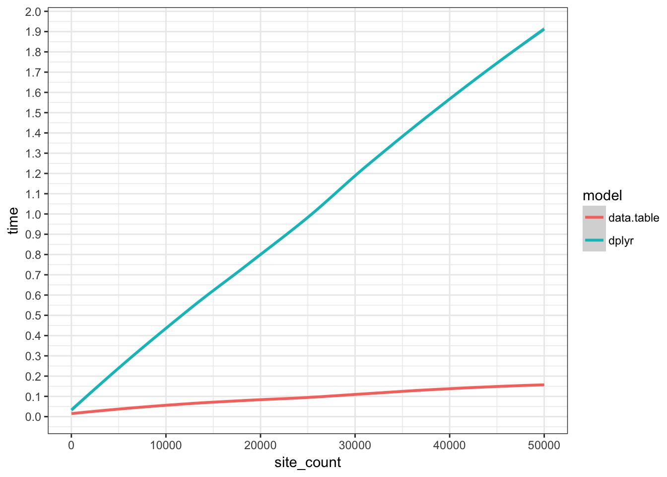
“site_count” is a measure of the simulation size (i.e. size of the data.frames). Then some costly, but not absurd calculations are performed on the data.
Why is data.table faster?
- optimized for speed
- Modifies “by reference”
tidyverse functions instead “copy-on-modify”.
Modify by reference vs. copy
Copy-on-modify
- Creates a copy of the data
- Modifies the copy
- Returns the copy
Modify-in-place (modify “by reference”)
- References the data
- Modifies the original data
Avoids duplicating data, which is costly for your computer’s memory, especially with large datasets.
Modify by reference vs. copy
You may have noticed that I had to add an extra call to print data.tables after modifying them.
This is because the line dt[, y := c("a", "b")] doesn’t return anything.
Because it edited the data in place, not by creating a copy.
Dangers of editing by reference
Modifying by reference can be dangerous if you are not careful.
What happens to “dt” if we remove a column from “dt2”?
“dt” and “dt2” reference the same underlying data.
Dangers of editing by reference
If you truly want a new copy of a data.table, use
Even Faster!
Keys
Keys provide some organization to your data.
This makes it much faster to later:
filter
group by
merge
data.table lets you add keys in a variety of ways.
You can also pass a vector of keys c("x", "y") to use.
What are keys?
Keys provide an index for the data.
Think of this like a phone book.
If you wanted to look my phone number up in the phone book,
you would search under “D” for DeHaven
you would not search the entire phone book!
When we tell data.table to use some columns as a key, it presorts and indexes the data on those columns.
Merging with data.table
For data.table all types of merges are handled by one function:
dt <- data.table(x = c("a", "b", "c"), y = 1:3)
dt2 <- data.table(x = c("a", "c", "d"), z = 4:6)
merge(dt, dt2, by = "x")
Key: <x>
x y z
<char> <int> <int>
1: a 1 4
2: c 3 5By default, merge() does an “inner” join (matches in both datasets).
Merging with data.table
A “left” join,
Or an “outer” join
Non-matching column names
We can also be explicit about which columns to use from “x” and from “y”,
dt <- data.table(x = c("a", "b", "c"), y = 1:3)
dt2 <- data.table(XX = c("a", "c", "d"), z = 4:6)
merge(dt, dt2, by.x = "x", by.y = "XX")
Key: <x>
x y z
<char> <int> <int>
1: a 1 4
2: c 3 5But it’s probably better to clean up your column names before hand.
data.table pivots
A package tidyfast which offers
dt_pivot_longer()dt_pivot_wider()
to match the syntax of tidyr but with the speed of data.table.
tidyverse or data.table?
tidyverse or data.table?
In practice, I (and many people) use a mix of both.
I personally prefer data.tables syntax for filtering, modifying columns, and summarizing.
If you really want the speed of data.table and the syntax of dplyr…
dtplyr
…there is a special package that combines the two!
dtplyr allows you to use all of the tidyverse verbs:
mutate()filter()groupby()
But behind the scenes runs everything using data.table.
A note on pipes
You can use pipes with data.table as well.
The underscore character _ is known as a “placeholder”,
and represents the object being piped.
A bit less useful because the data.table syntax is already very short.
Summary
renv- Separate libraries
snapshot()packages to lockfiles
- Introduced to
data.table- Using square bracket positions
dt[i, j, by=] - Fast and concise
- Keys
merge()melt()anddcast()
- Using square bracket positions
Live Coding Example
- Loading
data.table
Coding Exercise
- Install and load
data.tablein a temporary workspace - Create a
data.tablewith columnsaandbof length 10 with random values - Add new column
cwhich is the sum ofaandb - Add a new column
dwhich is the product ofaandbwhenais greater than 0