<?xml version="1.0" encoding="utf-8" ?>
<seriess realtime_start="2024-02-19" realtime_end="2024-02-19">
<series id="UNRATE" realtime_start="2024-02-19" realtime_end="2024-02-19" title="Unemployment Rate" observation_start="1948-01-01" observation_end="2024-01-01" frequency="Monthly" frequency_short="M" units="Percent" units_short="%" seasonal_adjustment="Seasonally Adjusted" seasonal_adjustment_short="SA" last_updated="2024-02-02 07:49:02-06" popularity="94" notes="The unemployment rate represents the number of unemployed as a percentage of the labor force. Labor force data are restricted to people 16 years of age and older, who currently reside in 1 of the 50 states or the District of Columbia, who do not reside in institutions (e.g., penal and mental facilities, homes for the aged), and who are not on active duty in the Armed Forces. This rate is also defined as the U-3 measure of labor underutilization. The series comes from the 'Current Population Survey (Household Survey)' The source code is: LNS14000000"/>
</seriess>R Databases and APIs
Connecting to data remotely
February 26, 2025
Lecture Summary
Downloading data
Introduction to APIs
fredrtidycensus- Mapping with
sf
Introduction to Databases
dbplyr- Example: WRDS
Downloading Data
Downloading Data
You have likely downloaded data from online for a project.
Perhaps you went to FRED.
- hosted by the St. Louis FED
- hosts a bunch of US time series
And let’s say you downloaded the time series for unemployment.
Downloading Unemployment Data from FRED
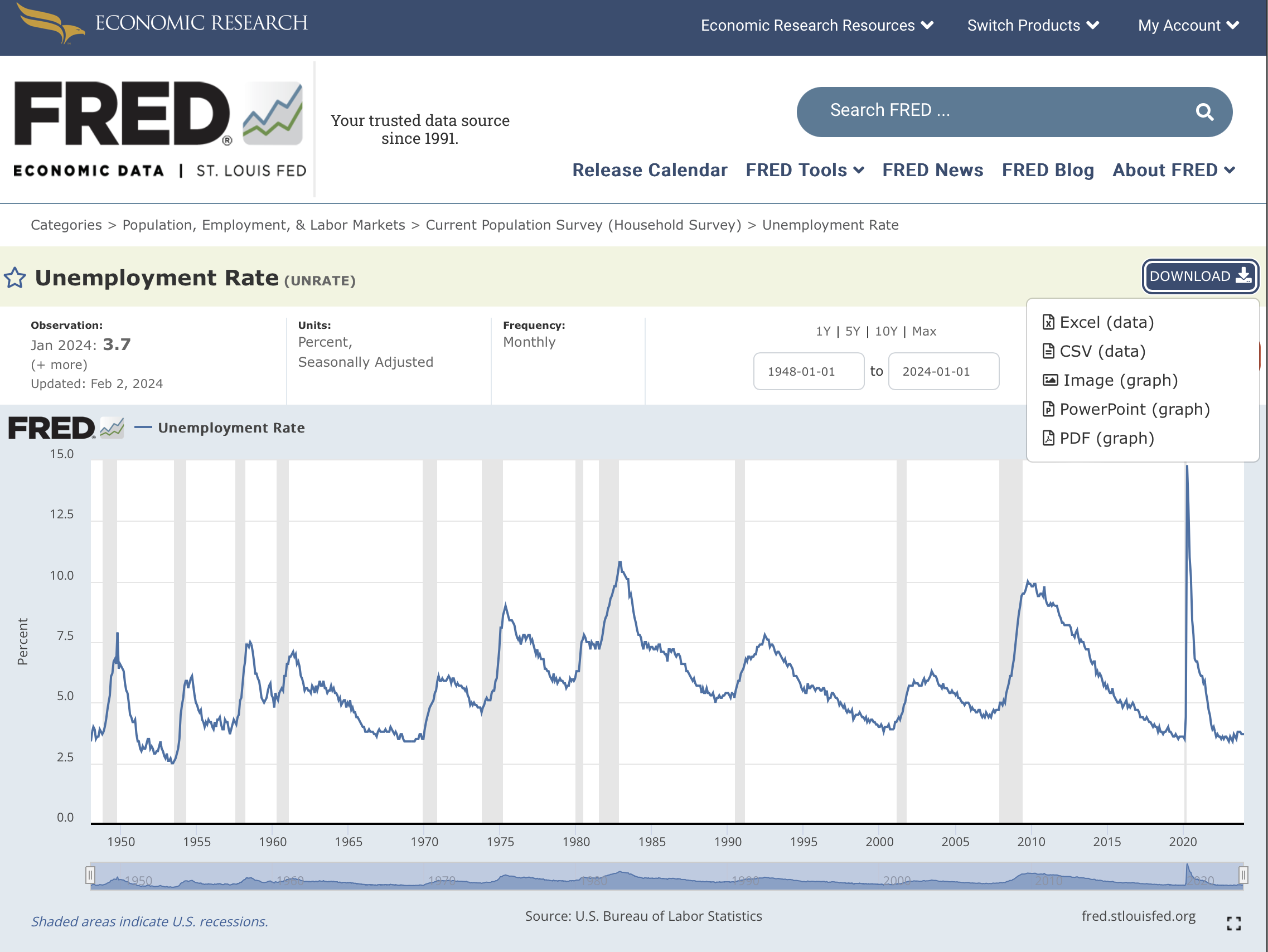
Downloading Unemployment Data from FRED
Once you have selected your file type (say csv),
You copy the file into your project’s raw data folder.
Then you can write a script to clean the data, merge it with your other datasets, etc.
Communicating Data Download Instructions
How might you record your data aquisition for replicability?
- Go to https://fred.stlouisfed.org
- Search for “Unemployment”
- Select “Unemployment Rate” from results
- Click the blue “Download” button
- Choose the “CSV” option from the dropdown
- Copy the “UNRATE.csv” file into the raw-data folder
- Run “clean-unrate.r” to clean the data
Overly Descriptive?
These may seem overly descriptive.
You could just say, “Downloaded unemployment rate from FRED”.
But this is a bit unclear about which unemployment rate you downloaded.
And for other data sources, the steps to get to the correct series and “download” button may be quite difficult for someone to replicate without explicit instructions.
A Better Option?
Instead of having to choose between:
- short, unclear data acquisition documentation
- long, cumbersome data acquisition documentation
We can use FRED’s API.
APIs
What is an API?
API stands for “application programing interface”.
- It details how a program will talk to other programs.
For us, APIs determine how data servers will respond to requests for data.
I think it’s easiest to contrast it with the UI or “user interface”:
- UIs: how programs respond to human requests
- APIs: how programs respond to other program requests
Requesting Data from a Server
When you go to FRED and click on “Unemployment Rate” you are sending a request over “https”
The server is going to send you back a nice “html” webpage because you are a human.
Instead, we could ask for the same series from the API…
And we would get an error asking for an API key (think password)…
API Keys
You have to authenticate yourself when working with an API.
A specific api key like: “abcdefghijklmnopqrstuvwxyz123456”
- unique value to you
Servers require this because they want to limit how many requests they get from one individual.
You can overwhelm an API with requests.
If you do, they will shut off your API key (and you’ll have to get a new one).
For FRED, you can get an api key here.
Requesting Data from an API
Adding an API key (this one is fake)
We would get a response that looks like this!
<seriess realtime_start="2024-02-19" realtime_end="2024-02-19">
<series id="UNRATE" realtime_start="2024-02-19" realtime_end="2024-02-19" title="Unemployment Rate" observation_start="1948-01-01" observation_end="2024-01-01" frequency="Monthly" frequency_short="M" units="Percent" units_short="%" seasonal_adjustment="Seasonally Adjusted" seasonal_adjustment_short="SA" last_updated="2024-02-02 07:49:02-06" popularity="94" notes="The unemployment rate represents the number of unemployed as a percentage of the labor force. Labor force data are restricted to people 16 years of age and older, who currently reside in 1 of the 50 states or the District of Columbia, who do not reside in institutions (e.g., penal and mental facilities, homes for the aged), and who are not on active duty in the Armed Forces. This rate is also defined as the U-3 measure of labor underutilization. The series comes from the 'Current Population Survey (Household Survey)' The source code is: LNS14000000"/>
</seriess>Which is just the metadata for the unemployment rate series.
Requesting the Actual Data Observations
If we wanted the actual data observations, we’d have to adjust our request to
<observations realtime_start="2024-02-19" realtime_end="2024-02-19" observation_start="1600-01-01" observation_end="9999-12-31" units="lin" output_type="1" file_type="xml" order_by="observation_date" sort_order="asc" count="913" offset="0" limit="100000">
...
<observation realtime_start="2024-02-19" realtime_end="2024-02-19" date="2023-08-01" value="3.8"/>
<observation realtime_start="2024-02-19" realtime_end="2024-02-19" date="2023-09-01" value="3.8"/>
<observation realtime_start="2024-02-19" realtime_end="2024-02-19" date="2023-10-01" value="3.8"/>
<observation realtime_start="2024-02-19" realtime_end="2024-02-19" date="2023-11-01" value="3.7"/>
<observation realtime_start="2024-02-19" realtime_end="2024-02-19" date="2023-12-01" value="3.7"/>
<observation realtime_start="2024-02-19" realtime_end="2024-02-19" date="2024-01-01" value="3.7"/>
</observations>
I trimmed the response here, it was about 1000 rows.
Making API Requests from R
You can request any webpage from R using the RCurl package
RCurl::getURL("https://api.stlouisfed.org/fred/series?series_id=UNRATE&api_key=abcdefghijklmnopqrstuvwxyz123456")And our response would look something like this:
Cleaning the Response
Now that we can make our request, we have to parse it and clean it to a format we want to use.
- FRED by default returns “XML” responses.
- Another common type of response is “JSON”.
Both of these can just be thought of as different types of lists.
If you find yourself making requests directly to an API, I suggest using the httr2 package. It has a great article about APIs.
But luckily for us, someone has already written a package to make and parse requests to FRED!
fredr: FRED API Wrapper for R
I wanted you to see the internals of how an API works, but usually if there is an API, someone has made a wrapper package to communicate with it.
For FRED and R: fredr
Then we can load the package, and importantly, set our api key.
Requesting FRED Data Directly from R
Now, let’s download that unemployment data.
# A tibble: 924 × 5
   date       series_id value realtime_start realtime_end
   <date>     <chr>     <dbl> <date>         <date>
 1 1948-01-01 UNRATE      3.4 2025-01-10     2025-01-10
 2 1948-02-01 UNRATE      3.8 2025-01-10     2025-01-10
 3 1948-03-01 UNRATE      4   2025-01-10     2025-01-10
 4 1948-04-01 UNRATE      3.9 2025-01-10     2025-01-10
 5 1948-05-01 UNRATE      3.5 2025-01-10     2025-01-10
 6 1948-06-01 UNRATE      3.6 2025-01-10     2025-01-10
 7 1948-07-01 UNRATE      3.6 2025-01-10     2025-01-10
 8 1948-08-01 UNRATE      3.9 2025-01-10     2025-01-10
 9 1948-09-01 UNRATE      3.8 2025-01-10     2025-01-10
10 1948-10-01 UNRATE      3.7 2025-01-10     2025-01-10
# ℹ 914 more rows
And we get a tibble as a reponse!
Combining Multiple Requests
fredr suggests we use the purrr::map_dfr() function to get multiple series.
Combining Multiple Requests
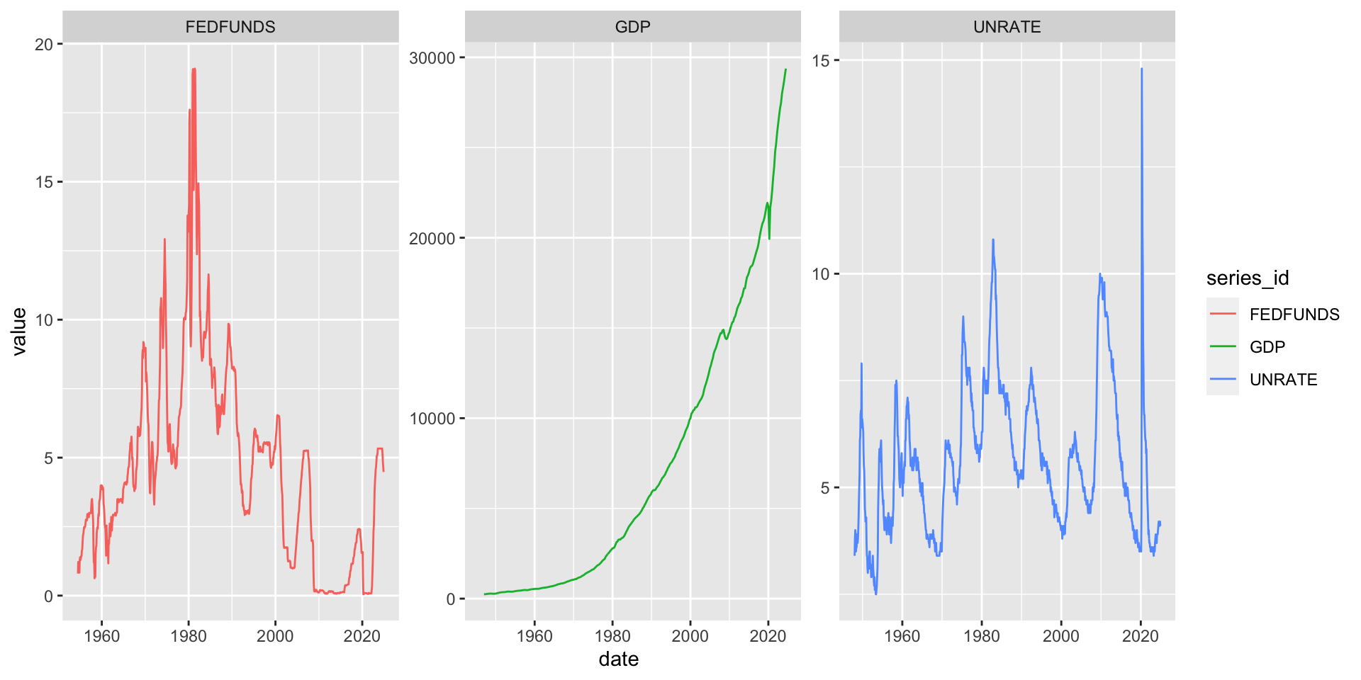
fredr Options
You can pass additional arguments to your FRED API request.
- start or end date
- frequency
- standard transformations
- pct change, year-over-year change, differences, etc.
- vintage values
Benefits of using an API for Data
- Self Documenting
- Programs are explicit about exactly what data you requested
- Faster
- Especially if you decide to download one more series for a robustness check
- But even just getting data, it takes literally two lines of R code
APIs Can Work the Other Way
We won’t be using this, but you can also send information to a server through an API.
For instance,
- Twitter has an API
- You could ask the API for your most recent tweets
- Or you could send the API the tweet you would like to send out.
See the package rtweet if you want to try this out.
Another API: tidycensus
I want to show you an example of one more API, for the Cesnus.
In fact, this package goes above and beyond, by automatically merging census data onto the right shapefiles for you.
- i.e. if you ask for state-level data, it will return the shapefiles for all US states
Setting up tidycensus
Just like before, you will need an API key. You can get one here.
Again, if you are commiting to a public repository, you should not commit your API key.
Requesting Data
tidycensus has many different functions for requesting different census data.
Here’s an example pulling data from the American Community Survey
- survey of a sample US households every year
- “B19013_011” is the Census code for “median household income”
- We set “geometry = TRUE” because we want the shapefiles as well
SF Data
Notice that the shapefile data is just a data.frame, with a bit of extra information.
[1] "sf" "data.frame"Simple feature collection with 250 features and 5 fields (with 3 geometries empty)
Geometry type: MULTIPOLYGON
Dimension: XY
Bounding box: xmin: -71.86277 ymin: 41.14634 xmax: -71.12057 ymax: 42.0188
Geodetic CRS: NAD83
First 10 features:
GEOID NAME variable
1 44001030100 Census Tract 301, Bristol County, Rhode Island B19013_001
2 44003021600 Census Tract 216, Kent County, Rhode Island B19013_001
3 44003020101 Census Tract 201.01, Kent County, Rhode Island B19013_001
4 44005040800 Census Tract 408, Newport County, Rhode Island B19013_001
5 44007014100 Census Tract 141, Providence County, Rhode Island B19013_001
6 44007010200 Census Tract 102, Providence County, Rhode Island B19013_001
7 44007000400 Census Tract 4, Providence County, Rhode Island B19013_001
8 44007011800 Census Tract 118, Providence County, Rhode Island B19013_001
9 44007011100 Census Tract 111, Providence County, Rhode Island B19013_001
10 44007001200 Census Tract 12, Providence County, Rhode Island B19013_001
estimate moe geometry
1 99167 11319 MULTIPOLYGON (((-71.3539 41...
2 130104 25333 MULTIPOLYGON (((-71.39157 4...
3 71932 7447 MULTIPOLYGON (((-71.53322 4...
4 72209 10138 MULTIPOLYGON (((-71.31293 4...
5 39652 16124 MULTIPOLYGON (((-71.45225 4...
6 51349 9094 MULTIPOLYGON (((-71.38557 4...
7 43456 25844 MULTIPOLYGON (((-71.42086 4...
8 48259 17241 MULTIPOLYGON (((-71.44129 4...
9 31393 4611 MULTIPOLYGON (((-71.40705 4...
10 40380 6980 MULTIPOLYGON (((-71.43134 4...Subsetting SF Data
We can use our dplyr verbs on this “sf” object as well.
Simple feature collection with 1 feature and 5 fields
Geometry type: MULTIPOLYGON
Dimension:     XY
Bounding box:  xmin: -71.40973 ymin: 41.82205 xmax: -71.39999 ymax: 41.83571
Geodetic CRS:  NAD83
        GEOID                                                NAME   variable
1 44007003602 Census Tract 36.02, Providence County, Rhode Island B19013_001
  estimate   moe                       geometry
1   145189 46476 MULTIPOLYGON (((-71.40973 4...
This is the census tract where we are in right now.
Plotting SF Data
And with ggplot2, it is extremely easy to plot!
Plotting SF Data
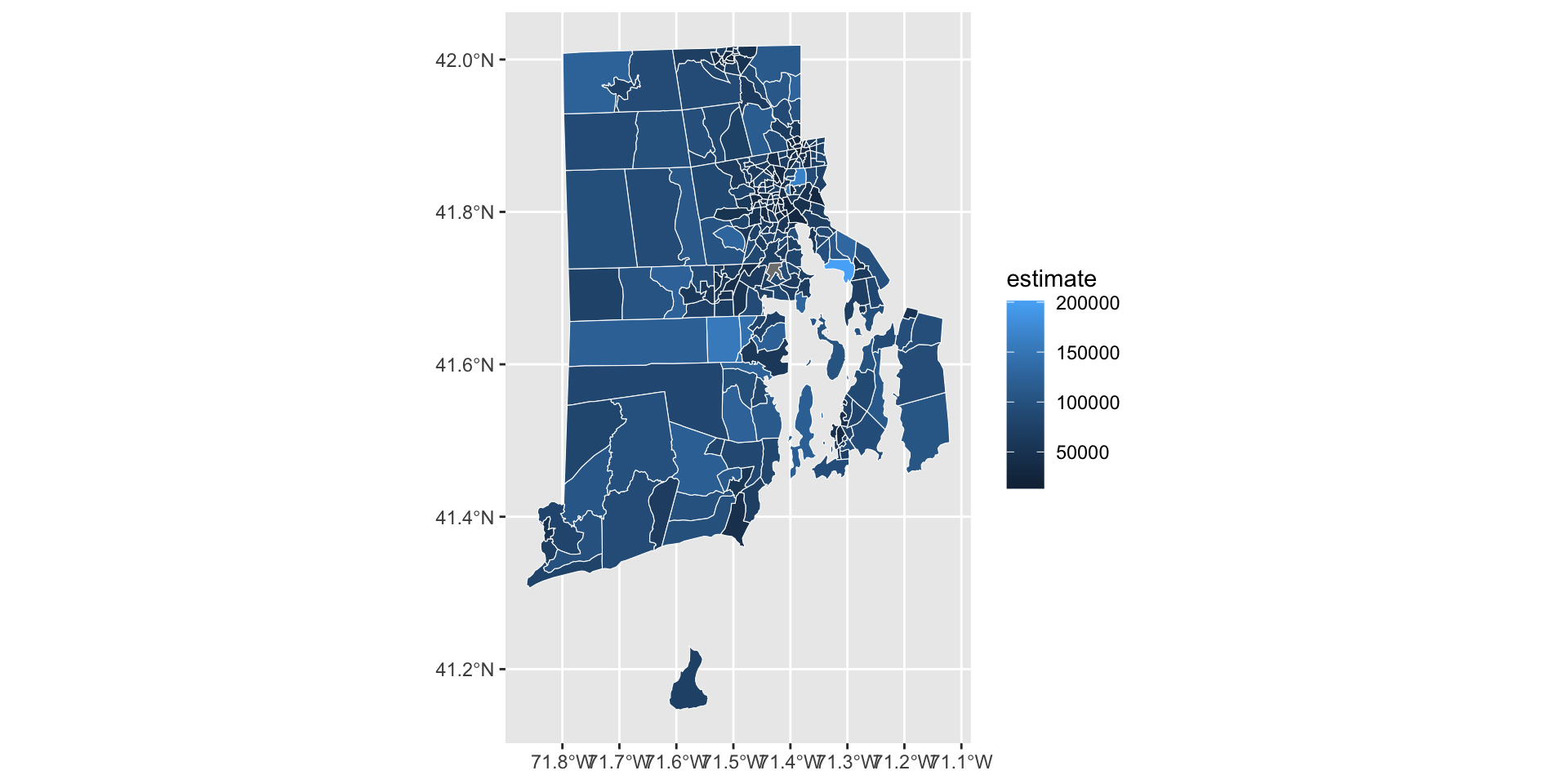
Plotting SF Data Interactive
We can use the package mapview for an interactive html map.
It is simple to call it on our sf data.
Plotting SF Data Interactive
API Summary
Incredibly useful for downloading data quickly.
Improves the flexibility of your code.
- i.e. you can add new data series more easily
Improves the reproducibility of your project.
Sadly, not all data sources have an API. ☹️
Databases
Intro to Databases
Databases are
- remote or local, but usually remote
- small or big, but usually big
- usually written in SQL
- “Structured Query Language”
Remember when we talked about setting “keys” for a dataset?
Databases take this to the extreme by heavily structuring the data.
A Database Consists of Tables
Here’s an example database, with multiple linked tables:
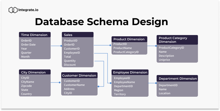
How is a Database Different than an API?
Both are sources where you can access data.
APIs
- Only return the requested data.
Databases
- Can perform expensive calculations for you before returning the data
- i.e. merging large tables, filtering, summarizing, etc.
Querying Databases with SQL
As I said before, almost every database runs on SQL.
- This is its own programming language.
You Don’t Need to Learn SQL
Luckily for all of us, we do not need to learn SQL to query a database.
We can use dbplyr!
This is a backend for—you guessed it—dplyr that translates dplyr verbs into SQL queries for us!
This is what we will be using to query a database.
Finding a Database to Query
Databases are not as readily accesible as APIs.
- Remember, they are performing computations for you, so they are more expensive to set up and maintain.
We will be accessing databases hosted by WRDS.
This requires you to have a personal account, which you can get throgh the Brown Library.
It will be optional on the assignment to make a WRDS account. It takes a couple days to get approved.
Connecting to a Database in R
The instructions for connecting to a database will usually be documented by the host.
In this case, WRDS tells us that their SQL database uses Postgress SQL and can be connected to with the following code:
Specifying a Table
Remember, a database is a bunch of tables.
We are going to ask for the table that stores the Dow Jones Index at a daily frequency.
# Source:   table<djdaily> [?? x 9]
# Database: postgres  [mdehaven@wrds-pgdata.wharton.upenn.edu:9737/wrds]
   date         djc  djct   dji  djit   djt  djtt   dju  djut
   <date>     <dbl> <dbl> <dbl> <dbl> <dbl> <dbl> <dbl> <dbl>
 1 1896-05-26    NA    NA  40.9    NA    NA    NA    NA    NA
 2 1896-05-27    NA    NA  40.6    NA    NA    NA    NA    NA
 3 1896-05-28    NA    NA  40.2    NA    NA    NA    NA    NA
 4 1896-05-29    NA    NA  40.6    NA    NA    NA    NA    NA
 5 1896-06-01    NA    NA  40.6    NA    NA    NA    NA    NA
 6 1896-06-02    NA    NA  40.0    NA    NA    NA    NA    NA
 7 1896-06-03    NA    NA  39.8    NA    NA    NA    NA    NA
 8 1896-06-04    NA    NA  39.9    NA    NA    NA    NA    NA
 9 1896-06-05    NA    NA  40.3    NA    NA    NA    NA    NA
10 1896-06-08    NA    NA  39.8    NA    NA    NA    NA    NA
# ℹ more rows
How Big is the Table?
One way to figure out the size of a table would be to download all the data.
This could be very bad. These datasets can be huge!
Instead, let’s ask the database how big the table is, and what min and max dates are,
Writing a Query
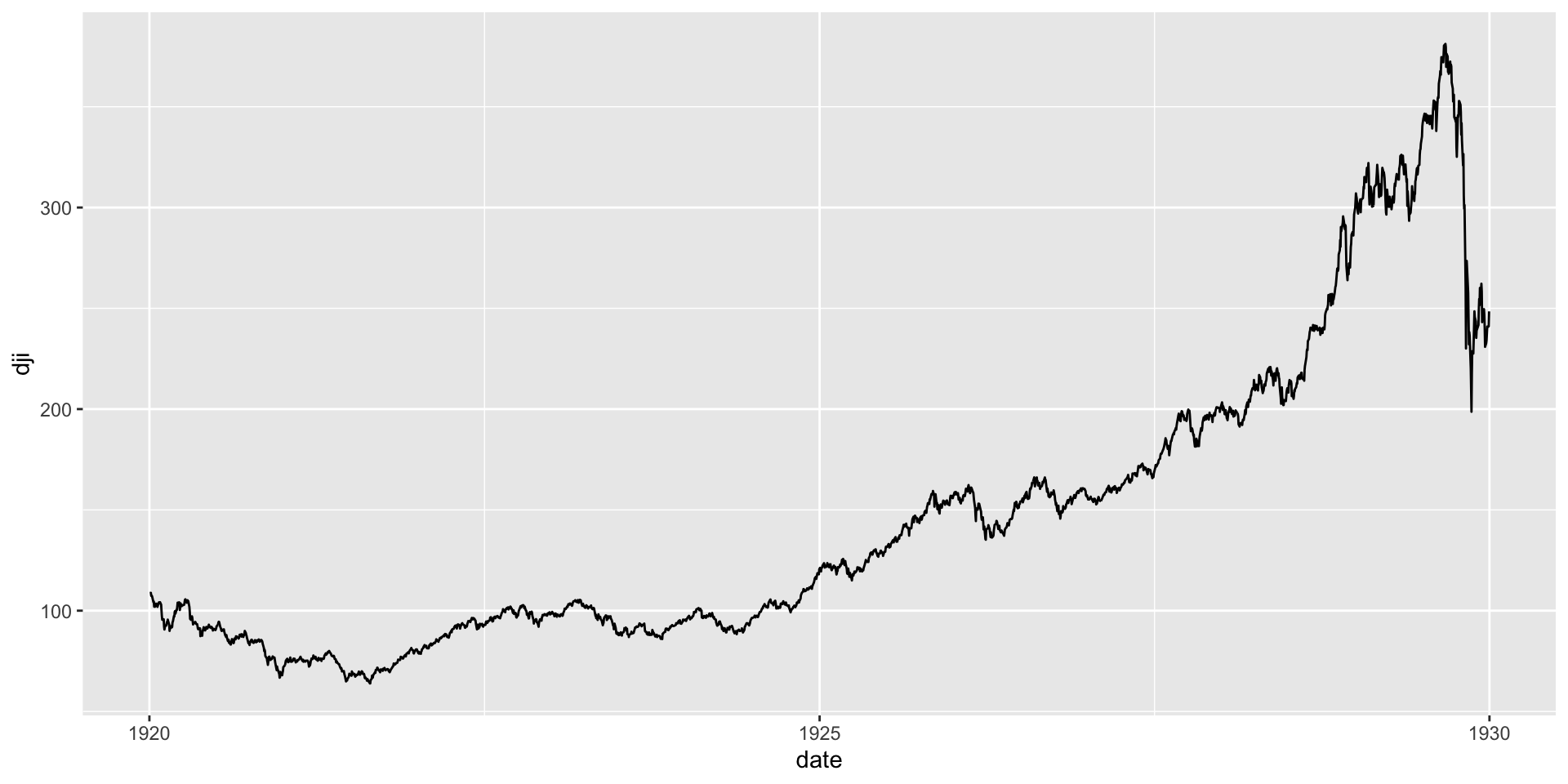
Let’s grab the data for the 1920s, just for the columns we want.
- We can write this with our
dplyrverbs, as if it was a “tibble”
query <- dj_db |>
  filter(date >= as.Date("1920-01-01")) |>
  filter(date <= as.Date("1930-01-01")) |>
  select(date, dji)
query
# Source: SQL [?? x 2]
# Database: postgres [mdehaven@wrds-pgdata.wharton.upenn.edu:9737/wrds]
date dji
<date> <dbl>
1 1920-01-02 109.
2 1920-01-05 109.
3 1920-01-06 107.
4 1920-01-07 108.
5 1920-01-08 107.
6 1920-01-09 107.
7 1920-01-12 104.
8 1920-01-13 105.
9 1920-01-14 102
10 1920-01-15 104.
# ℹ more rowsNotice, we still are not getting all of the data, just the first few observations.
Collecting the Data
Once you have your full query written and you are confident you can handle the data size, you should add |> collect().
This will actually execute the full query and return all of the results.
data <- dj_db |>
  filter(date >= as.Date("1920-01-01")) |>
  filter(date <= as.Date("1930-01-01")) |>
  select(date, dji) |>
  collect()
data
# A tibble: 2,502 × 2
date dji
<date> <dbl>
1 1920-01-02 109.
2 1920-01-05 109.
3 1920-01-06 107.
4 1920-01-07 108.
5 1920-01-08 107.
6 1920-01-09 107.
7 1920-01-12 104.
8 1920-01-13 105.
9 1920-01-14 102
10 1920-01-15 104.
# ℹ 2,492 more rowsPlotting the DJI in the 1920s
A Bigger Table
The DJI table was on the small side. Let’s take a look at the size of this CRSP table instead:
# Source:   SQL [1 x 1]
# Database: postgres  [mdehaven@wrds-pgdata.wharton.upenn.edu:9737/wrds]
        n
  <int64>
1 5037353
Over 5 million observations!
This is monthly data, for each stock.
Operations We Perform
You could probably still work with 5 million observations on your local machine.
But what if you wanted to merge all the stock observations with a table of company balance sheet information?
That would be a pretty taxing merge for your computer.
But it would be easy for the database to handle.
dbplyr Query Translation
If you would like, you can ask dbplyr to show you the SQL translation for your queries.
<SQL>
SELECT "date", "dji"
FROM "djones"."djdaily"
WHERE
  ("date" >= CAST('1920-01-01' AS DATE)) AND
  ("date" <= CAST('1930-01-01' AS DATE))
This can be a good way to pick up some SQL, or to troubleshoot queries that aren’t working as expected.
Why are Databases Faster?
Databases are much faster than doing the same calculations on your own computer.
- Their servers are much, much larger
- The data is sctructured/organized when in the database
Once you collect the data to your machine, it is just a normal data.frame, no organization.
Database summary
You will not find many databases out in the wild for you to query.
But if you do find one for your data, use it.
They are how most companies store internal data.
And knowing some SQL is often a requirement for data science jobs.
Summary
Lecture Summary
- Data acquisition is a hard to document research step
- Accessing data remotely and programatically has benefits
- for reproducibility
- for speed
- for big data
- Example APIs
fredrtidycensus- You can make cool maps in R
- Example Database:
- WRDS
Live Coding Example
Coding Exercise
- Request a FRED API key here
- Use the following “http” structure to request a series through your browser
https://api.stlouisfed.org/fred/series/observations?series_id=UNRATE&api_key=abcdefghijklmnopqrstuvwxyz123456- Use the
Rcurl::getURL()function to make the same request through an R session