library(tidyverse)
library(ggplot2)
library(patchwork)R ggplot2 Example
Loading Packages
We are going to load the tidyverse to use a few data manipulation tools.
Data
The ggplot2 package comes with a small economics dataset that we will use.
economics# A tibble: 574 × 6
date pce pop psavert uempmed unemploy
<date> <dbl> <dbl> <dbl> <dbl> <dbl>
1 1967-07-01 507. 198712 12.6 4.5 2944
2 1967-08-01 510. 198911 12.6 4.7 2945
3 1967-09-01 516. 199113 11.9 4.6 2958
4 1967-10-01 512. 199311 12.9 4.9 3143
5 1967-11-01 517. 199498 12.8 4.7 3066
6 1967-12-01 525. 199657 11.8 4.8 3018
7 1968-01-01 531. 199808 11.7 5.1 2878
8 1968-02-01 534. 199920 12.3 4.5 3001
9 1968-03-01 544. 200056 11.7 4.1 2877
10 1968-04-01 544 200208 12.3 4.6 2709
# ℹ 564 more rowsEconomic Variable Definitions
- pce personal consumption expenditures, in bilions of dollars
- pop total population, in thousands
- psavert personal savings rate
- empmed median duration of unemployment, weeks
- unemploy number of unemployed, thousands
Plotting Unemployment
urate_plot <-
  economics |>
  mutate(urate = 100 * (unemploy / pop)) |>
  ggplot(aes(
    x = date,
    y = urate
  )) +
  geom_line()
urate_plot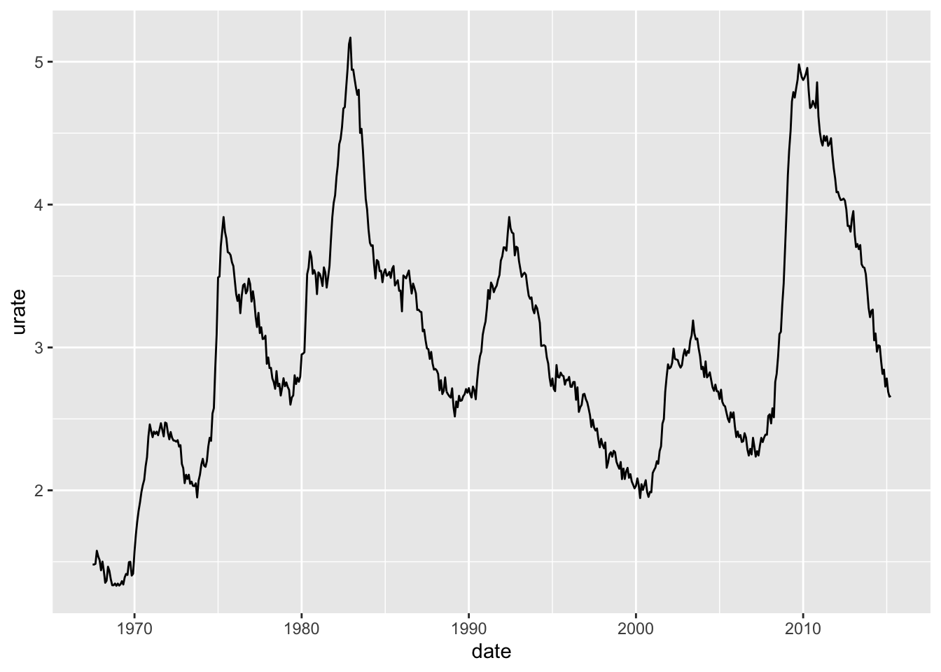
This doesn’t look right! Wasn’t the unemployment rate ~ 10% during the 08-09 recession?
Yes. We calculated the unemployment rate out of the total U.S. population, when the official statistic is calculated from the labor force population (i.e. 18+, looking for a job, etc.).
Creating our own theme
Let’s create our own theme to use on all of our plots. It’s easiest to start with prebuilt theme that’s close to what you want, but I am going to list everything out just as an example.
my_theme <-
  # theme_bw() +  ## Normally you'd start from a default you like
  theme(
    panel.background = element_rect(fill = "cornsilk", color = "wheat"),
    panel.grid.major = element_line(color = "wheat"),
    panel.grid.minor = element_blank()
  )
Notice the three element_ calls.
Many theme arguments take a specific element depending on what they are—backgrounds are rectangles, the grids are lines, axes are also lies, text is text.
Each element_ call has further arguments controlling its colors, fills, lineweights, etc.
Also, you can always pass an element_blank() to theme argument to simply remove that visual object. We did that for the minor grid (the ticks between the labeled tick marks).
And here is how it looks:
urate_plot <- urate_plot + my_theme
urate_plot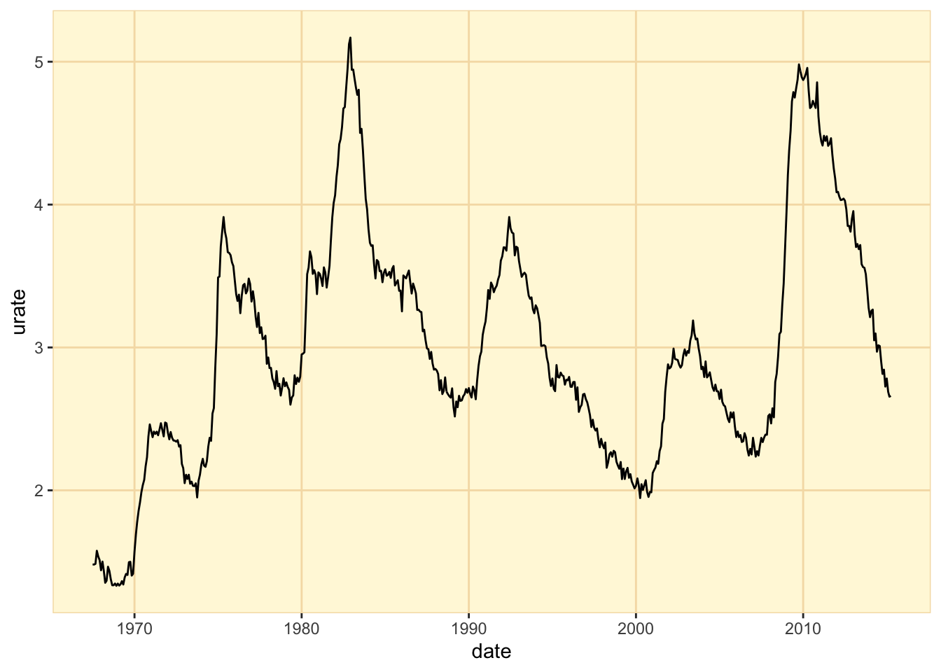
Creating a Chartpack
Let’s say we want a chartpack of the 08-09 recession using our economics data.
We should calculate what the inflation rate is, and maybe show how it changes along with the savings rate, then print everything out to a pdf.
economics <- economics |> mutate(infrate = 100 * (pce / lag(pce, 12) - 1))inf_plot <-
economics |>
ggplot(aes(
x = date
)) +
geom_line(aes(y = infrate)) +
geom_line(aes(y = psavert)) +
my_theme
inf_plot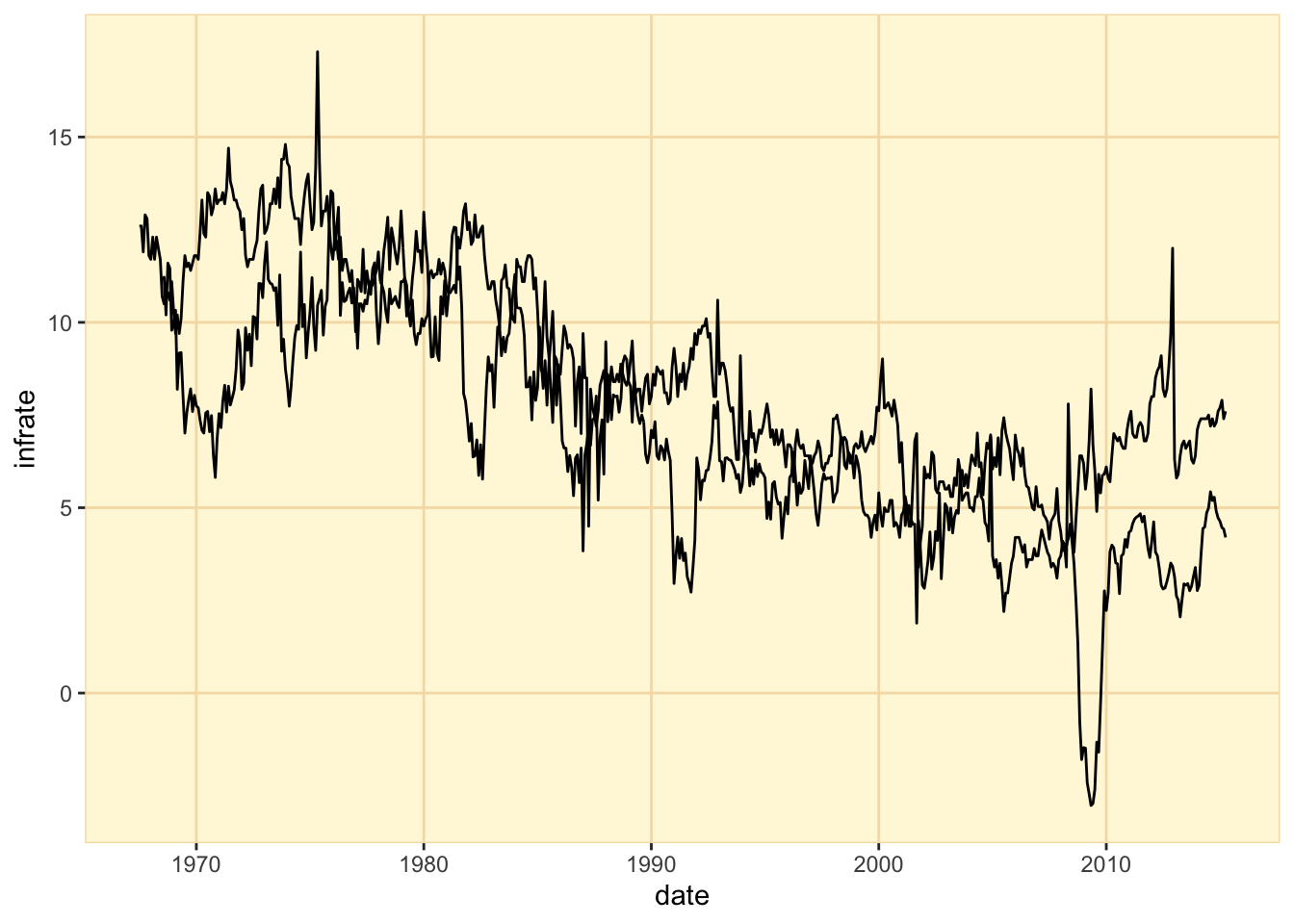
We need to set a color aesthetic to be able to distinguish the two lines. While we are at it, we will go ahead and add a color scale.
inf_plot <-
  economics |>
  ggplot(aes(
    x = date
  )) +
  geom_line(aes(y = infrate, color = "Inflation")) +
  geom_line(aes(y = psavert, color = "Savings Rate")) +
  scale_color_manual(values = c(Inflation = "steelblue", `Savings Rate` = "lightblue")) +
  my_theme
inf_plot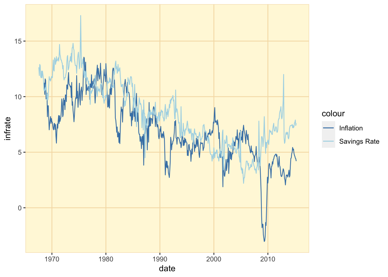
Looks like there is a big time trend down for both, but what’s the actual correlation between the two?
scatter_plot <-
  economics |>
  ggplot(aes(
    x = infrate,
    y = psavert
  )) +
  geom_point() +
  geom_smooth(method = "lm", se = FALSE, color = "firebrick") +
  my_theme
scatter_plot
It would be nice to actually label the correlation between the two series on the plot.
This is where the annotate function is very handy. It lets you draw a single instance of a geom, without needing to reference your data.
corr_val <- cor(economics$infrate, economics$psavert, use = "complete")

scatter_plot <- scatter_plot +
  annotate("text", x = -2, y = 17, label = round(corr_val, 4), color = "firebrick")
scatter_plot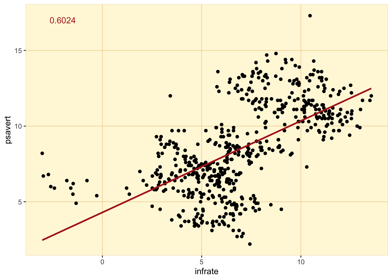
Combine all the plots
comb_plot <- urate_plot + inf_plot + scatter_plot + guide_area() + plot_layout(guides = "collect")
comb_plot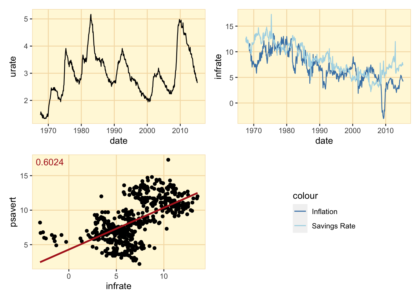
Saving to a pdf
Finally, let’s save it out as full page of a pdf.
ggsave("test-ggplot-chartpack.pdf", comb_plot, width = 7.5, height = 10, units = "in")